12 One Proportion
In the bootstrap chapter we met a medical consultant who advertises that her clients have fewer complications than the national average: 3 complications in 62 liver-donor surgeries, against a national rate of about 10%. Is she really better than average? Or would another 62 of her patients tell a different story?
Every result would come out differently with new data. This chapter asks how differently, for a single proportion, in three steps: simulate what chance alone produces, model it with a formula that skips the simulation, and compare the two to learn when the formula can be trusted.
12.1 The question
Let \(p\) be the consultant’s true complication rate, the rate we would see over all the patients she could ever advise. Her sample rate is
\[\hat{p} = \frac{3}{62} = 0.048,\]
about half the national 10%. But 62 patients is not many, and complication counts bounce around from one group of patients to the next. The question is whether a rate this low could easily come from an average consultant:
- \(H_0\): her true rate is the national rate, \(p = 0.10\).
- \(H_A\): her true rate is lower, \(p < 0.10\).
The bootstrap chapter noted that her stronger claim, that her work causes fewer complications, can’t be settled with these data: patients who hire a consultant may differ in other ways. Here we ask only whether her rate is lower.
12.2 Simulate
12.2.1 A world where she is average
In the randomization tests chapter we compared two groups by shuffling their labels. Here there is only one group and a claimed value, \(p = 0.10\), so there is nothing to shuffle. Instead we build the null world directly: imagine thousands of patients, 10% of whom have a complication, and draw 62 of them at a time. Each draw is one simulated study by an average consultant.
Predict → Do → Explain.
- Predict. An average consultant expects about \(62 \times 0.10 \approx 6\) complications in 62 surgeries. How often would she get 3 or fewer just by chance: about 1 study in 100, 1 in 20, or 1 in 5?
- Do. Open the one-proportion randomization test. It is set to the null world (\(p = 0.10\)) and to “less than.” Add 1,000 simulated studies.
- Explain. What share of the simulated studies had a rate at or below her 0.048? Would her record stand out among 1,000 average consultants?
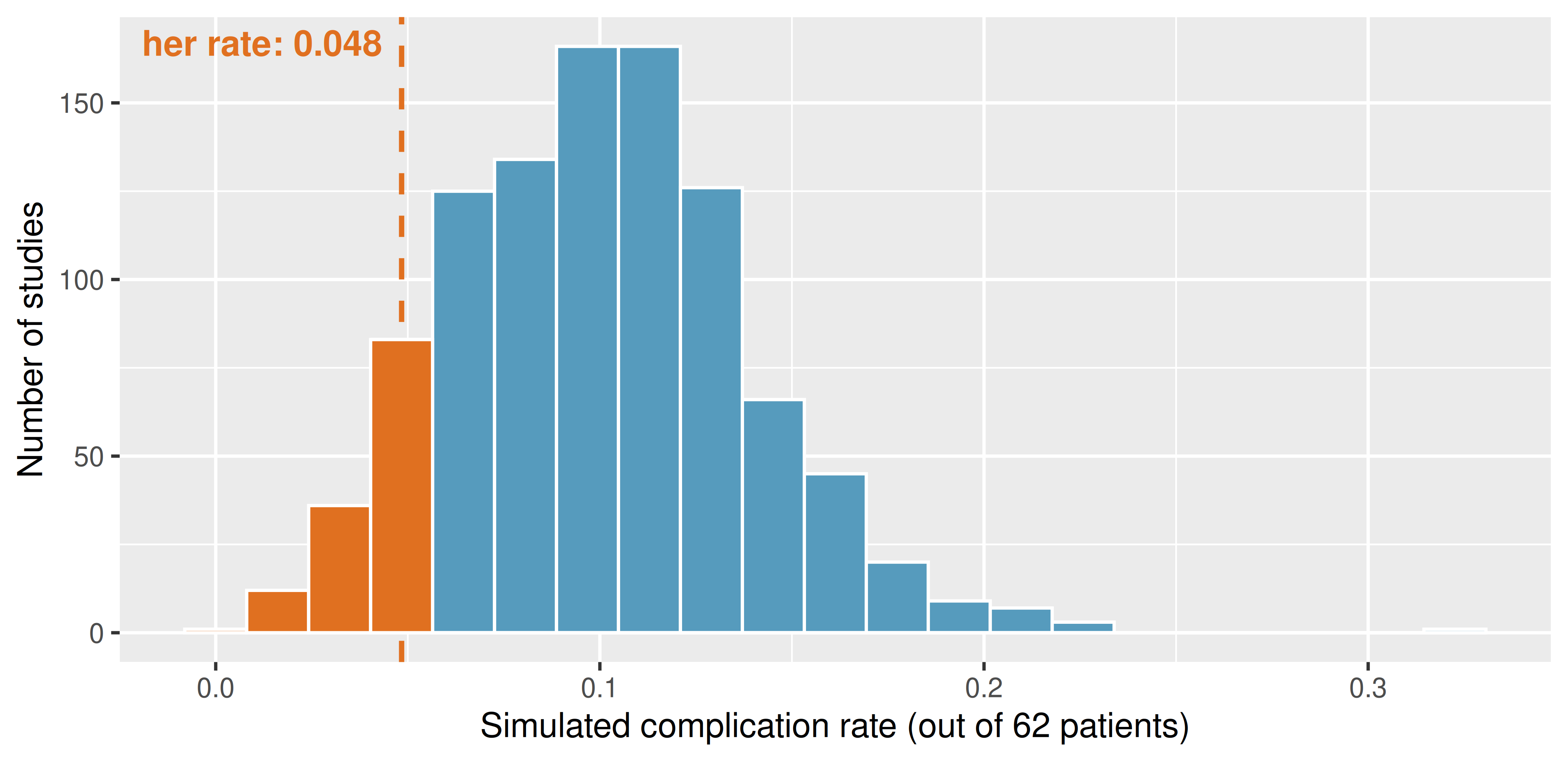
About 13% of the simulated studies, roughly 1 in 8, did as well as she did or better, with nothing special going on. That is the \(p\)-value. Her record is not unusual for an average consultant, so we do not have convincing evidence that her true rate is below 10%. (Your StatLens run will give a slightly different share, about 12%. That difference is simulation error, which the randomization tests chapter showed shrinks as you run more simulations.)
12.2.2 The interval
The bootstrap chapter estimated her true rate the other way, by resampling her 62 patients. The 95% bootstrap interval ran from 0.000 to 0.113: plausible true rates from 0% up to about 11%.
The national 10% sits inside that interval, which is the same message the test gave. A value inside the interval is one we would not reject; we come back to this connection in the Compare section.
We did not reject \(p = 0.10\). Does that mean her true rate is 10%?
No. Failing to reject means the data are compatible with 10%, not that 10% is correct. The interval says her true rate could be anywhere from about 0% to 11%: much better than average, about average, or a little worse. With only 62 patients, the data can’t tell these apart.
12.3 Model
12.3.1 A shortcut for the null distribution
The simulation needed a computer and a thousand studies. Look again at Figure 12.1: the simulated rates have a center (at the null value, 0.10) and a typical spread, and the shape is roughly a hill. The sampling distributions chapter showed that the normal curve often models a pile of simulated statistics like this one. If it fits, we can skip the simulation.
The center is the null value \(p_0\). The spread has a formula:
\[SE = \sqrt{\frac{p_0\,(1 - p_0)}{n}} = \sqrt{\frac{0.10 \times 0.90}{62}} = 0.038.\]
The standard deviation of our 1,000 simulated rates was 0.039, close to the formula’s 0.038. The formula is describing the same spread the simulation produced.
A normal model for \(\hat{p}\). When the conditions below hold, the sample proportion \(\hat{p}\) from a sample of size \(n\) behaves approximately like a normal distribution with
- center: the true proportion \(p\);
- spread: \(SE = \sqrt{p\,(1-p)/n}\).
12.3.2 The \(z\) test
To read a \(p\)-value off the normal model, measure how far \(\hat{p}\) is from the null value in standard errors:
\[z = \frac{\hat{p} - p_0}{SE_0}, \qquad SE_0 = \sqrt{\frac{p_0\,(1 - p_0)}{n}}.\]
The \(p\)-value is the area beyond \(z\) under the standard normal curve, in the direction of \(H_A\). Use \(p_0\) in the standard error because a test asks what would happen if \(H_0\) were true.
Predict → Do → Explain.
- Predict. In Figure 12.1 the simulated rates are lopsided: they pile up against 0 on the left and trail off to the right. Will the normal curve’s \(p\)-value come out smaller than, larger than, or about the same as the simulation’s 1 in 8?
- Do. Open the one-proportion \(z\) test. It opens on the consultant’s data; check that the null value is 0.10 and choose the “less than” alternative, then read the \(p\)-value.
- Explain. How far is the normal answer from the simulation’s? Keep the number in mind for the Compare section.
Compute the \(z\) test for the consultant.
\(SE_0 = 0.038\) (above), so
\[z = \frac{0.048 - 0.10}{0.038} = -1.35.\]
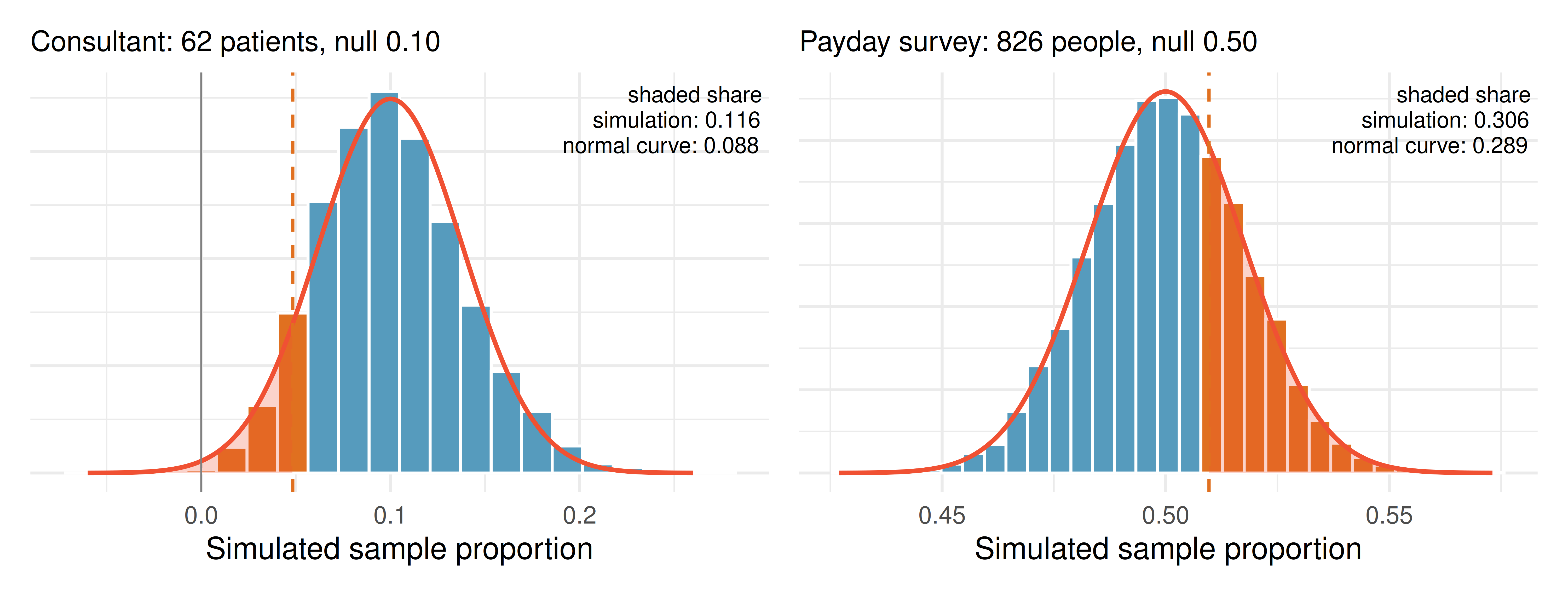
The area to the left of \(z = -1.35\) is 0.088. That is noticeably smaller than the simulation’s 1 in 8 (about 0.12). Same data, different answers. The Compare section explains why.
12.3.3 The confidence interval
A confidence interval uses the same shape around the sample’s own estimate, so its standard error uses \(\hat{p}\):
Confidence interval for one proportion.
\[\hat{p} \pm z^* \times \sqrt{\frac{\hat{p}\,(1-\hat{p})}{n}}\]
with \(z^* = 1.645\) for 90%, \(1.96\) for 95%, and \(2.576\) for 99% confidence.
For the consultant, \(SE = \sqrt{0.048 \times 0.952 / 62} = 0.027\), and the 95% interval is
\[0.048 \pm 1.96 \times 0.027 = (-0.005,\ 0.102).\]
The lower end is negative, a complication rate below zero. Something is off.
12.3.4 When the shortcut works
The normal model is an approximation, and it needs two conditions:
- Independence. The observations are independent of one another, for example a random sample, or patients whose outcomes don’t affect each other.
- Success–failure. Enough successes and failures that the pile of possible \(\hat{p}\) values is close to a symmetric hill: at least 10 expected of each.
- For a test, use the null value: \(np_0 \ge 10\) and \(n(1-p_0) \ge 10\).
- For an interval, use the estimate: \(n\hat{p} \ge 10\) and \(n(1-\hat{p}) \ge 10\).
The consultant fails both versions: \(np_0 = 62 \times 0.10 = 6.2\) expected complications under \(H_0\), and only 3 observed.
12.4 Compare
12.4.1 Same data, different answers
Here is everything we have for the consultant, side by side.
| \(p\)-value (\(H_A\): \(p < 0.10\)) | 95% interval for \(p\) | |
|---|---|---|
| Simulation, six runs of 1,000 studies | 0.105 to 0.127 | bootstrap: (0.000, 0.113) |
| Simulation, six runs of 10,000 studies | 0.118 to 0.128 | |
| Normal model | 0.088 | (-0.005, 0.102) |
Could the gap between the simulation and the normal model just be simulation error? Rerun the simulation and see. Six runs of 1,000 studies landed between 0.105 to 0.127. Six runs of 10,000 landed between 0.118 to 0.128. More simulations steady the answer near 0.12, and none of the runs comes close to 0.088. The simulation is consistent; the normal model is the one that’s off.
Going deeper: where does StatLens’s ± come from?
The share of simulated studies that land in the tail is itself a sample proportion: out of \(N\) simulated studies, some fraction \(\hat{p}_{\text{sim}}\) were at least as extreme as the data. So it has a standard error, and it is this chapter’s formula with \(N\), the number of simulated studies, in place of \(n\):
\[SE_{\text{sim}} = \sqrt{\frac{\hat{p}_{\text{sim}}\,(1 - \hat{p}_{\text{sim}})}{N}}.\]
For the consultant, a share near 0.125 from \(N = 1{,}000\) studies gives \(SE_{\text{sim}} = \sqrt{0.125 \times 0.875 / 1000} = 0.010\). StatLens reports \(1.96 \times SE_{\text{sim}} \approx 0.020\), the “± 0.020” beside its \(p\)-value. Because \(N\) is under a square root, 10,000 studies cut the simulation error by a factor of \(\sqrt{10} \approx 3\), to about ± 0.006.
Notice what is not in the formula: the consultant’s 62 patients. Simulation error depends on \(N\), how many studies we simulate, never on \(n\), the size of her sample. More simulations make our estimate of the \(p\)-value sharper; only more patients would make the evidence stronger.
Figure 12.2 shows why. With only about 6 complications expected, there are only a handful of possible rates (0/62, 1/62, 2/62, …), each one a big chunk of probability, bunched against zero. A smooth bell curve can’t match that lumpy, lopsided pile. Here it puts too little area at or below her 3 complications (0.088 against about 0.12), and it spreads into impossible negative rates. With 826 people and an expected 413 “yes” answers (right panel), the pile is smooth and symmetric, and the curve fits almost perfectly.
12.4.2 When the conditions hold: payday-loan borrowers
A random sample of 826 payday-loan borrowers was asked whether they would support a rule requiring lenders to check a borrower’s credit before making a loan. 421 (51%) said yes. Is there convincing evidence that a majority of borrowers support the rule?
- \(H_0\): \(p = 0.50\); \(H_A\): \(p > 0.50\).
- Conditions: a random sample, and \(np_0 = n(1-p_0) = 413\), well above 10.
| \(p\)-value (\(H_A\): \(p > 0.50\)) | 95% interval for \(p\) | |
|---|---|---|
| Simulation, six runs of 1,000 studies | 0.270 to 0.315 | bootstrap: (0.475, 0.544) |
| Normal model | 0.289 (\(z = 0.56\)) | (0.476, 0.544) |
This time the normal answer sits right among the simulation runs, and the two intervals match. That is what “the conditions hold” buys you: the formula gives the simulation’s answer without running it.
Run it yourself. Open the one-proportion randomization test, choose Enter Summary, and type 421 successes out of 826. Add 1,000 studies and compare the share with the table. Then do the same in the one-proportion \(z\) test (null value 0.50, “greater than”).
12.4.3 The interval and the test tell one story
The borrowers’ 95% interval runs from about 0.476 to 0.544. A confidence interval is the set of null values a two-sided test would not reject at the matching level.
Predict → Do → Explain.
- Predict. A two-sided test at the 5% level asks whether \(p\) differs from a null value. For the borrowers’ data, which of these null values would it reject: 0.46, 0.48, 0.50, 0.52, 0.54, 0.56? Use the interval.
- Do. In the randomization test, enter 421 out of 826, run 1,000 studies, and read the \(p\)-value. Change the null value and repeat.
- Explain. Which null values survived? Where are they relative to the interval?
Check your answer
| Null value | 0.46 | 0.48 | 0.50 | 0.52 | 0.54 | 0.56 |
|---|---|---|---|---|---|---|
| Two-sided \(p\)-value | 0.004 | 0.088 | 0.578 | 0.553 | 0.080 | 0.004 |
| Decision at 5% | reject | keep | keep | keep | keep | reject |
12.4.4 Which method should you use?
Choosing a route for one proportion.
- Check the conditions first. Independence, and at least 10 expected successes and failures.
- Conditions hold: the normal formulas are quick, and they give the simulation’s answer.
- Conditions fail: use a simulation (randomization test, bootstrap interval). The normal answer can be noticeably off, and an interval can even include impossible values.
- Any time: a simulation is a good check on a formula.
12.5 The four questions
A conclusion isn’t finished at “reject” or “don’t reject.” Here are both examples, answered in full.
The consultant (3 complications in 62 surgeries)
- Could it be chance? Yes. About 1 in 8 average consultants would do this well.
- How big is it? Her rate, 4.8%, is about half the national 10%, but the interval runs from 0% to about 11%. The data can’t distinguish “much better” from “about average.”
- Who does it apply to? Her past 62 clients, who are not a random sample of all the patients she might advise.
- Did one thing cause the other? Not from these data. This is an observational record, and her clients may differ from other patients in ways that matter.
The payday-loan borrowers (421 of 826 support credit checks)
- Could it be chance? Yes. A 51% “yes” is well within what an evenly split population produces (\(p \approx 0.29\)).
- How big is it? Support is somewhere between about 48% and 54%, close to an even split either way.
- Who does it apply to? Payday-loan borrowers like the ones sampled, since the sample was random.
- Did one thing cause the other? Not a causal question. This is a survey of opinions.
12.6 Chapter review
12.6.1 Summary
- Simulate. For one proportion, the null world is a population with the claimed rate \(p_0\). Draw samples of size \(n\) from it; the share of simulated studies at least as extreme as the data is the \(p\)-value. A bootstrap interval estimates \(p\) from the sample itself.
- Model. The sample proportion has an approximately normal sampling distribution with center \(p\) and \(SE = \sqrt{p(1-p)/n}\).
- Test: \(z = (\hat{p} - p_0)/\sqrt{p_0(1-p_0)/n}\).
- Interval: \(\hat{p} \pm z^* \sqrt{\hat{p}(1-\hat{p})/n}\).
- Compare. When there are at least 10 expected successes and failures (and the observations are independent), the formulas give the simulation’s answer. When there aren’t, they can be noticeably off, and simulation is the better route. A simulated answer has simulation error: rerunning moves it a little, and more simulations shrink it. It does not depend on the sample size.
- One story. A 95% interval holds the null values a two-sided 5% test would not reject.
- Four questions. A complete conclusion says whether it could be chance, how big the effect is, who it applies to, and whether anything caused it.
12.6.2 Key terms
Null value (\(p_0\)), one-proportion randomization test, normal model for \(\hat{p}\), standard error of \(\hat{p}\), \(z\) test for one proportion, confidence interval for one proportion, success–failure condition, simulation error.
12.6.3 Attribution
Adapted from Introduction to Modern Statistics, 2nd ed. (Çetinkaya-Rundel & Hardin), Chapter 16, “Inference for a single proportion” (CC BY-SA 3.0): the medical-consultant and payday-loan examples and the parametric-simulation approach. Reorganized for this book’s Simulate → Model → Compare structure; changes made.
12.7 Exercises
Warm-up
Quick practice with the vocabulary and mechanics, before the exercises. Answers are at the end. Each item’s MOM label (e.g. MOM 12.D17) is the same skill with new numbers, for more practice.
(MOM 12.D17) In a random sample of 390 adults, 257 said they prefer online shopping over in-store (\(\hat{p}\) = 0.659).
Test the hypotheses:
H₀: p = 0.7
Hₐ: p < 0.7Use a discernibility level of α = 0.01.
(a) Standard error (under H₀): ______
(b) Test statistic z: ______
(c) P-value: ______
(MOM 12.D18) In a random sample of 1350 adults, 540 said they believe college is worth the cost (\(\hat{p}\) = 0.4).
Construct a 99% confidence interval for the population proportion.
(a) Critical value z*: ______
(b) Standard error: ______
(c) Margin of error: ______
(d) Lower bound: ______
(e) Upper bound: ______
(MOM 12.D19) You want to test H₀: p = 0.6 with a sample of n = 135.
Are the conditions for using the normal approximation (z-procedure) satisfied?
- The conditions are met: np₀ = 81 ≥ 10 and n(1 − p₀) = 54 ≥ 10, and we are told the sample is random.
- The conditions are always met as long as the data come from a survey
- The conditions are not met because the sample size is too small.
- The conditions only require that n ≥ 30
(MOM 12.D20) A 90% confidence interval for the proportion of adults who support a policy is (0.49, 0.61).
Which of the following is the correct interpretation?
- There is a 90% probability that the true proportion is between 0.49 and 0.61
- 90% of all adults support the policy at a rate between 0.49 and 0.61
- We are 90% confident that the true population proportion of adults who support the policy is between 0.49 and 0.61
- If we repeated the survey, 90% of respondents would give the same answer
(MOM 12.D22) A researcher asks a random sample of adults whether they support the new policy, to test whether the proportion who support the new policy is greater than 0.50. The test produces a p-value of 0.03.
Using α = 0.05, what is the appropriate conclusion in context?
- The test is inconclusive and no statement can be made
- We accept H₀ and conclude that the population proportion is exactly the null value
- Since the p-value (0.03) is less than α = 0.05, we fail to reject H₀. There is not sufficient evidence.
- Since the p-value (0.03) is less than α = 0.05, we reject H₀. There is sufficient evidence to conclude that the proportion who support the new policy is greater than 0.50.
Warm-up answers
- 0.0232; -1.77; 0.0384
- 2.5758; 0.0133; 0.0343; 0.3657; 0.4343
- (a) The conditions are met: np₀ = 81 ≥ 10 and n(1 − p₀) = 54 ≥ 10, and we are told the sample is random.
- (c) We are 90% confident that the true population proportion of adults who support the policy is between 0.49 and 0.61
- (d) Since the p-value (0.03) is less than α = 0.05, we reject H₀. There is sufficient evidence to conclude that the proportion who support the new policy is greater than 0.50.
Note
Pilot draft. This chapter’s exercises will be regrouped from the one-proportion items in the current Inference for Proportions exercise set (IMS 16 and UWL 16-01 to 16-06) once the template chapter is approved.