17  Analysis of Variance

In earlier chapters, we developed methods to compare the mean of a quantitative outcome across two groups. An important aspect of those analyses was to look at the difference in sample means as an estimate for the difference in population means. When comparing more than two groups, simple subtraction will not fully capture the variation across three or more groups. As with two groups, the research question focuses on whether group membership is independent of the quantitative response variable. In this chapter, we focus on a new statistic that incorporates differences in means across more than two groups. Although the ideas are similar to the \(t\)-test, they have earned their own name: ANalysis Of VAriance, or ANOVA.

Sometimes we want to compare means across many groups. We might initially think to do pairwise comparisons. For example, if there were three groups, we might compare the first mean with the second, then with the third, and finally compare the second and third means – a total of three comparisons. However, this strategy can be treacherous. If we have many groups and do many comparisons, it is likely that we will eventually find a difference just by chance, even if there is no difference in the populations. Instead, we should apply a holistic test to check whether there is evidence that at least one pair of groups is different, which is where ANOVA saves the day.

ANOVA uses a single hypothesis test to check whether the means across many groups are equal:

• \(H_0\): The mean outcome is the same across all groups: \(\mu_1 = \mu_2 = \cdots = \mu_k\) where \(\mu_j\) represents the mean of the outcome for observations in category \(j\).
• \(H_A\): At least one mean is different.

Generally, we must check three conditions before performing ANOVA:

• The observations are independent within and between groups.
• The responses within each group are nearly normal.
• The variability across the groups is about equal.

When these conditions are met, we may perform ANOVA to determine whether the data provide convincing evidence against the null hypothesis.

College departments commonly run multiple sections of the same introductory course. Consider a statistics department that runs three sections of an intro stats course. We might like to determine whether there are substantial differences in first exam scores across sections A, B, and C. Describe appropriate hypotheses.

---

• \(H_0\): The average score is identical in all sections, \(\mu_A = \mu_B = \mu_C\). The observed differences are due to chance.
• \(H_A\): The average score varies by class. We would reject the null hypothesis if there were larger differences among the class averages than what we might expect from chance alone.

Strong evidence favoring the alternative hypothesis in ANOVA is described by unusually large differences among the group means. Assessing the variability of the group means relative to the variability among individual observations within each group is key to ANOVA’s success.

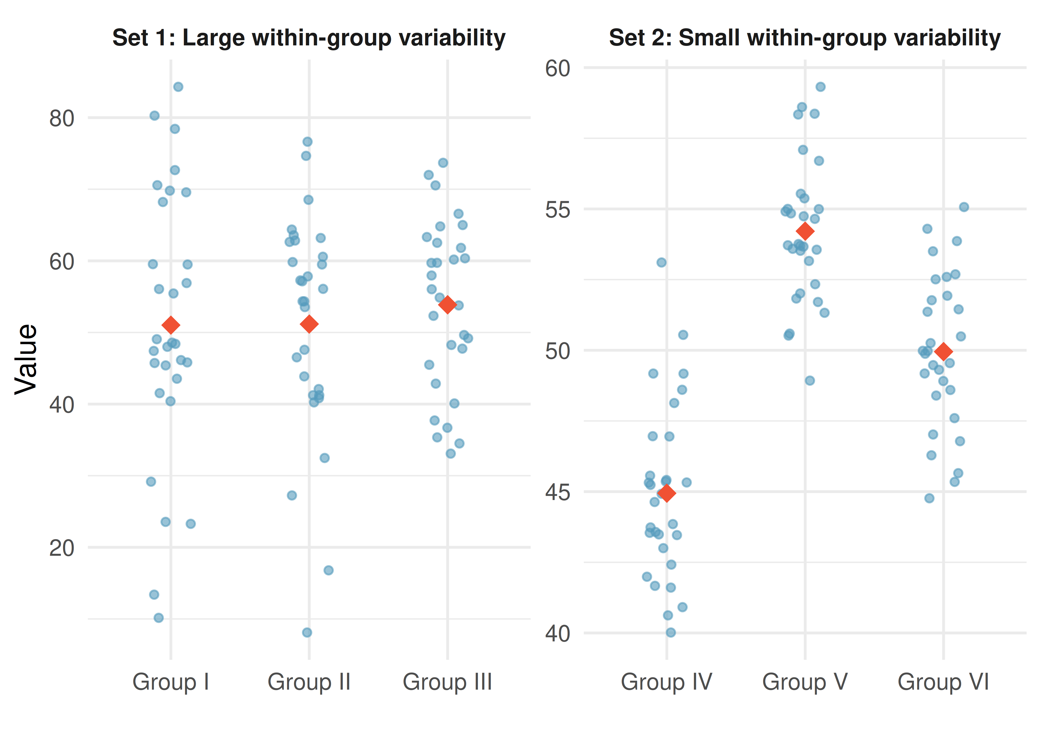
Consider the figure below showing two sets of three groups.

Figure 17.1: Side-by-side dot plots for two sets of three groups. In the first set (Groups I, II, III), the within-group variability is large relative to the between-group differences. In the second set (Groups IV, V, VI), the within-group variability is small and the between-group differences are clearly visible.

Compare Groups I, II, and III. Can you visually determine if the group differences are real? Now compare Groups IV, V, and VI.

---

Any real difference in Groups I, II, and III is difficult to discern because the data within each group are very volatile relative to differences in the group averages. On the other hand, Groups IV, V, and VI show noticeable differences because those differences are large relative to the variability in individual observations within each group.

17.1 Case study: MLB batting

We would like to determine whether there are real differences in batting performance among baseball players according to their position: outfielder (OF), infielder (IF), and catcher (C). We use data from 429 Major League Baseball players from the 2018 season who had at least 100 at-bats. The measure of batting performance is the on-base percentage (OBP), which roughly represents the fraction of the time a player successfully gets on base or hits a home run.

Summary statistics for each group:

Position	n	Mean	SD
OF	160	0.320	0.044
IF	205	0.318	0.037
C	64	0.302	0.038

Figure 17.2: Side-by-side box plots of on-base percentage for 429 players across three positions. The variability appears approximately constant across groups. Catchers seem to have a slightly lower on-base percentage.

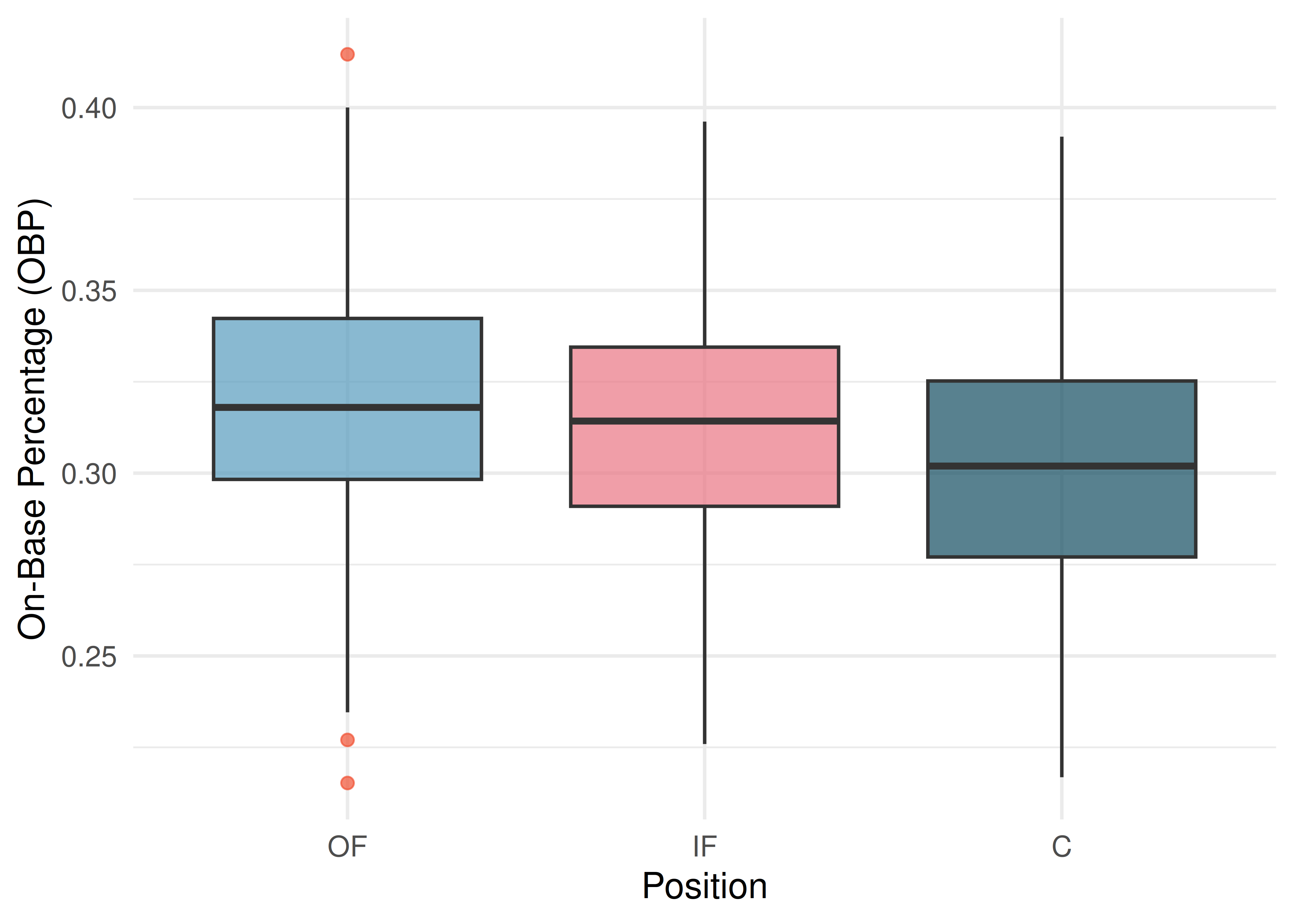
The null hypothesis under consideration is \(\mu_{OF} = \mu_{IF} = \mu_{C}\). Write the null and alternative hypotheses in plain language.

Show answer

\(H_0\): The average on-base percentage is equal across the three positions. \(H_A\): The average on-base percentage varies across some (or all) groups.

What would be an appropriate point estimate of the on-base percentage by outfielders, \(\mu_{OF}\)?

---

A good estimate of the on-base percentage by outfielders would be the sample average of OBP for just those players who are outfielders: \(\bar{x}_{OF} = 0.320\).

17.1.1 Why not just compare the most different groups?

The largest difference between sample means is between catchers and outfielders. Why might it be inappropriate to simply test whether \(\mu_C\) and \(\mu_{OF}\) are different?

---

The primary issue is data snooping (also called data fishing). We are inspecting the data before picking the groups to compare. It is inappropriate to examine all data informally and only afterward decide which parts to formally test. Naturally, we would pick the groups with the largest differences, which inflates the Type I error rate.

For example, suppose we measure aptitude for students in 20 classrooms where all students are randomly assigned. With so many groups, we will probably observe a few that look different just by chance. If we select only those classes and perform a formal test, we will probably reach the wrong conclusion.

17.2 Randomization test for comparing many means

17.2.1 The F-statistic

The method of analysis of variance focuses on answering one question: is the variability in the sample means so large that it seems unlikely to be from chance alone? We quantify the between-group variability using the mean square between groups (MSG), which has degrees of freedom \(df_G = k - 1\) where \(k\) is the number of groups. The MSG can be thought of as a scaled variance formula for the group means.

We also need a benchmark for how much variability to expect if the null hypothesis is true. For this, we compute the mean square error (MSE), which measures the variability within groups and has degrees of freedom \(df_E = n - k\).

The F-statistic is the ratio of these two quantities:

\[F = \frac{MSG}{MSE}\]

The MSG represents between-group variability, and MSE measures within-group variability. When the null hypothesis is true, any differences among sample means are due to chance, and the MSG and MSE should be about equal, making \(F\) close to 1. Large values of \(F\) suggest that the between-group differences are larger than what we would expect from random variation.

The test statistic for three or more means is an F.

The F statistic is a ratio of how the groups differ (MSG) as compared to how the observations within a group vary (MSE).

\[F = \frac{MSG}{MSE}\]

When the null hypothesis is true and the conditions are met, \(F\) has an F-distribution with \(df_1 = k - 1\) and \(df_2 = n - k\).

Conditions:

• Independent observations, both within and across groups
• Large samples and no extreme outliers

17.2.2 Variability of the statistic

Suppose we have three exams (A, B, and C) and want to investigate whether they differ in difficulty:

• \(H_0\): \(\mu_A = \mu_B = \mu_C\). The exams are equally difficult.
• \(H_A\): At least one exam is more (or less) difficult than the others.

Exam	n	Mean	SD	Min	Max
A	58	75.1	13.9	44	100
B	55	72.0	13.8	38	100
C	51	79.4	14.1	45	100

Figure 17.3: Box plots of exam scores for three exam versions. Exam C appears to have a higher median, but the distributions overlap.

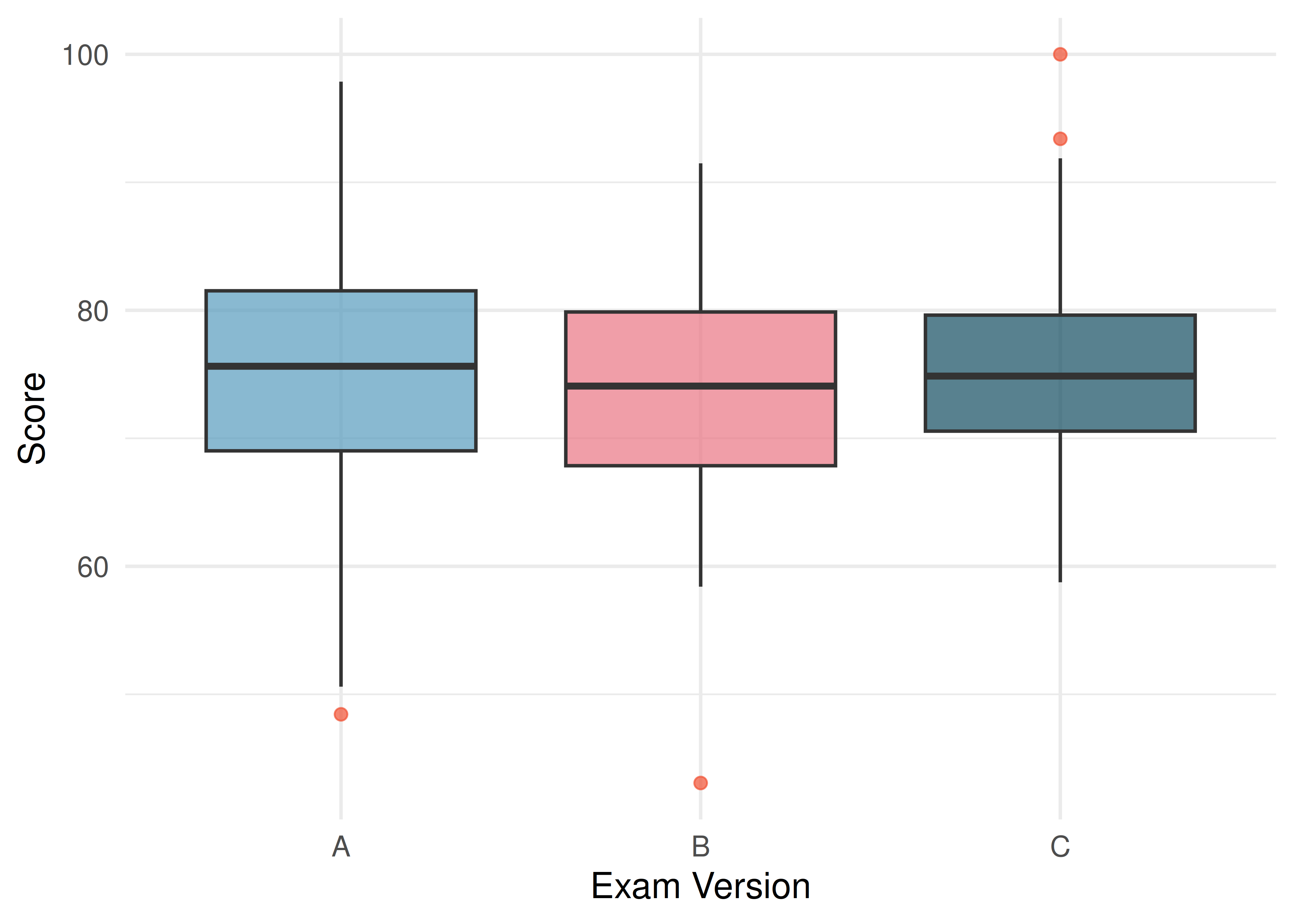
To perform a randomization test, we randomly reassign the exam labels to the observed scores. If the null hypothesis is true, the exam version should not matter, so any score could belong to any exam version.

Figure 17.4: The randomization process: exam version labels are randomly shuffled across the observed scores to generate a new assignment, from which a new F-statistic is computed. ↗ Try this live — shuffle the group labels yourself and see the resulting F-statistic.

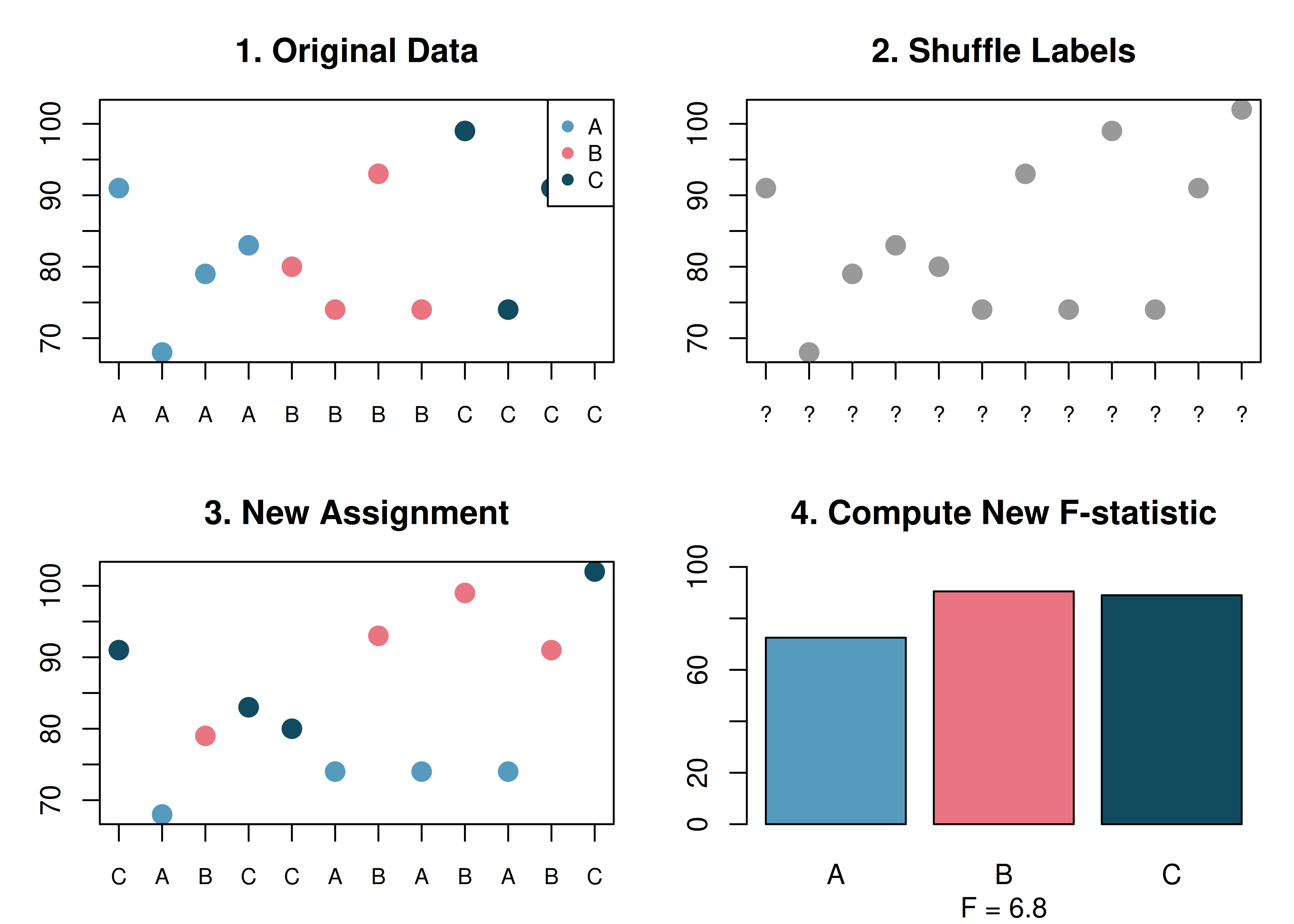
By repeating this process 1,000 times, we build a null distribution of F-statistics.

Figure 17.5: Histogram of F-statistics from 1,000 randomizations. The distribution is right-skewed with most values below 2. The tail extends to about 6. ↗ Try this live — build the null F distribution live — vary reps and watch it settle.

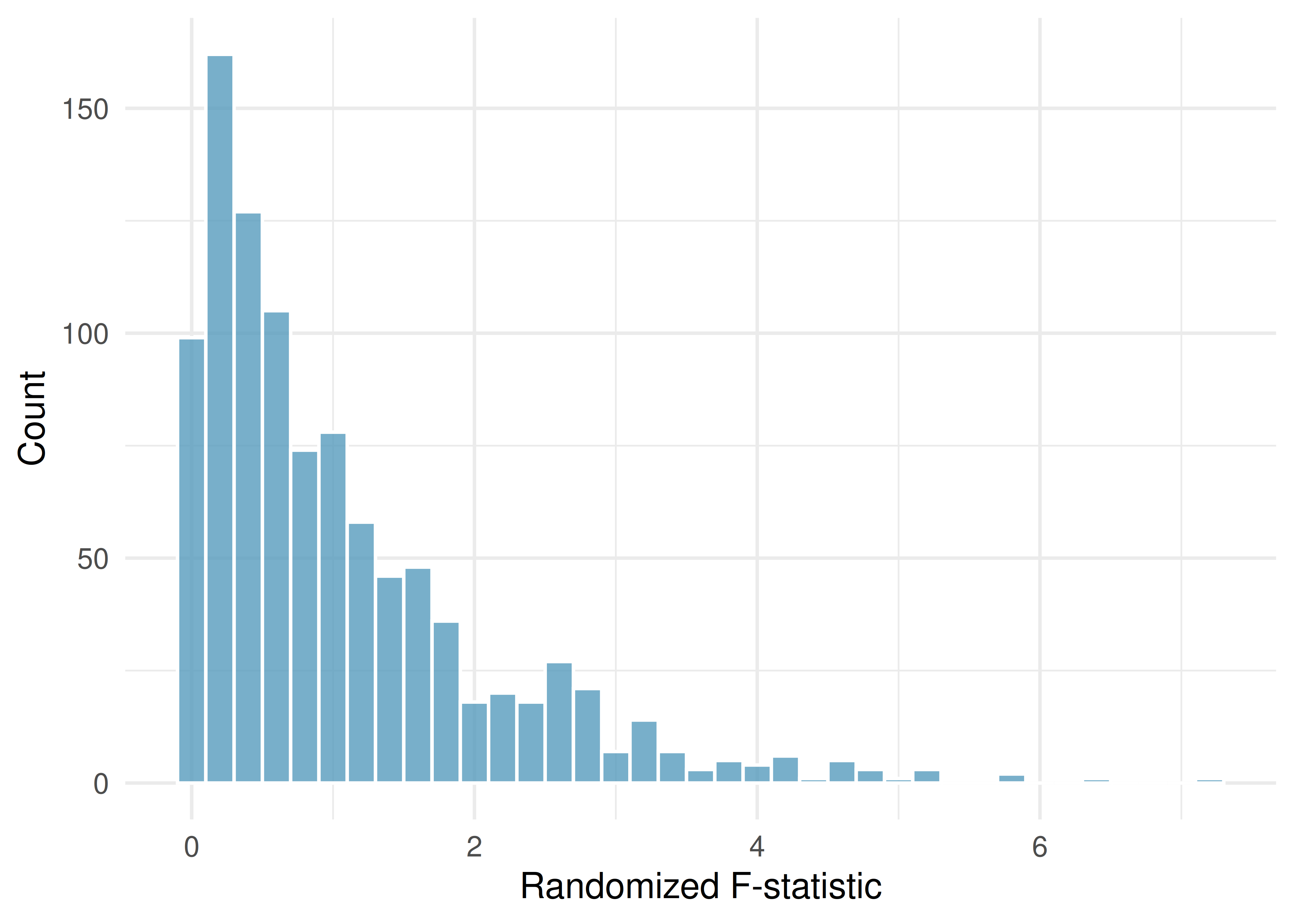
17.2.3 Observed statistic vs. null statistics

Figure 17.6: Histogram of F-statistics from 1,000 randomizations with the observed F-statistic of 3.48 marked by a red line. The area to the right represents the p-value. ↗ Try this live — reproduce the null distribution and place your observed F on it.

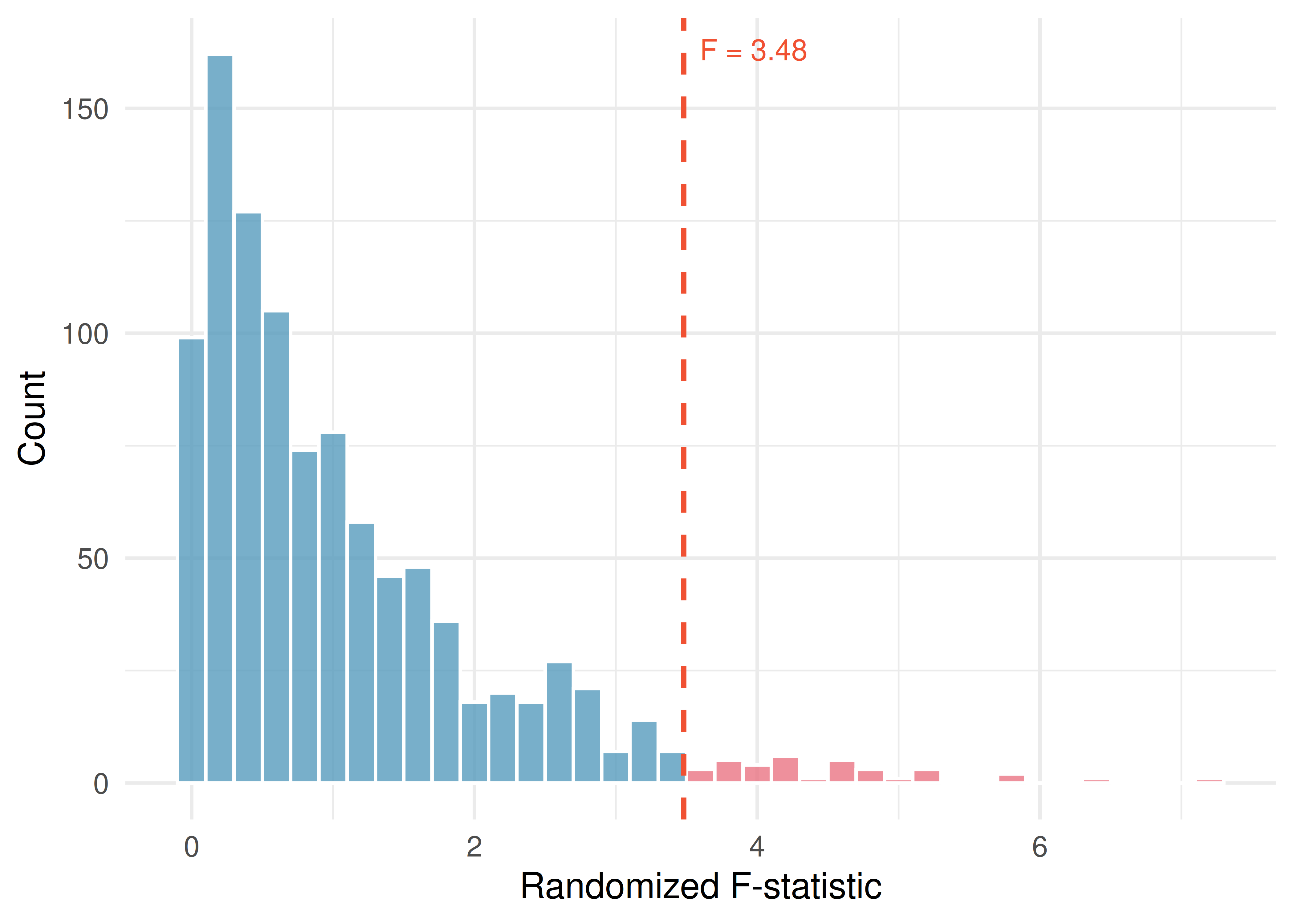
Using statistical software, we find that 3.6% of the randomized F statistics were at or above the observed test statistic of \(F = 3.48\). That is, the p-value is 0.036. Assuming a discernibility level of \(\alpha = 0.05\), the p-value is smaller than the discernibility level, which leads us to reject the null hypothesis. We conclude that the difficulty level is different for at least one of the exams.

17.3 Mathematical model for ANOVA

The randomization test on the F-statistic has a corresponding mathematical theory: the F-distribution.

17.3.1 Variability of the statistic

The larger the observed variability in the sample means (MSG) relative to the within-group variability (MSE), the larger the F-statistic and the stronger the evidence against the null hypothesis. We use the upper tail of the F-distribution to compute the p-value.

The F-statistic and the F-test.

Analysis of variance (ANOVA) uses a test statistic, the F-statistic, which represents a standardized ratio of variability in the sample means relative to the variability within the groups. If \(H_0\) is true and the model conditions are satisfied, the F-statistic follows an F-distribution with parameters \(df_1 = k - 1\) and \(df_2 = n - k\). The upper tail of the F-distribution is used to compute the p-value.

For the MLB data, \(MSG = 0.00803\) and \(MSE = 0.00158\). Identify the degrees of freedom associated with MSG and MSE and verify the F-statistic is approximately 5.077.

Show answer

There are \(k = 3\) groups, so \(df_G = k - 1 = 2\). There are \(n = 429\) total observations, so \(df_E = n - k = 426\). The F-statistic is \(F = \frac{MSG}{MSE} = \frac{0.00803}{0.00158} = 5.08 \approx 5.077\).

17.3.2 The p-value from the F-distribution

A p-value can be computed from the F-statistic using an F-distribution with \(df_1 = df_G\) and \(df_2 = df_E\).

Figure 17.7: An F-distribution with df₁ = 2 and df₂ = 426. The area to the right of F = 5.077 is shaded, representing a p-value of approximately 0.0066. ↗ Try this live — drag the cutline to any F value and read the right-tail p-value.

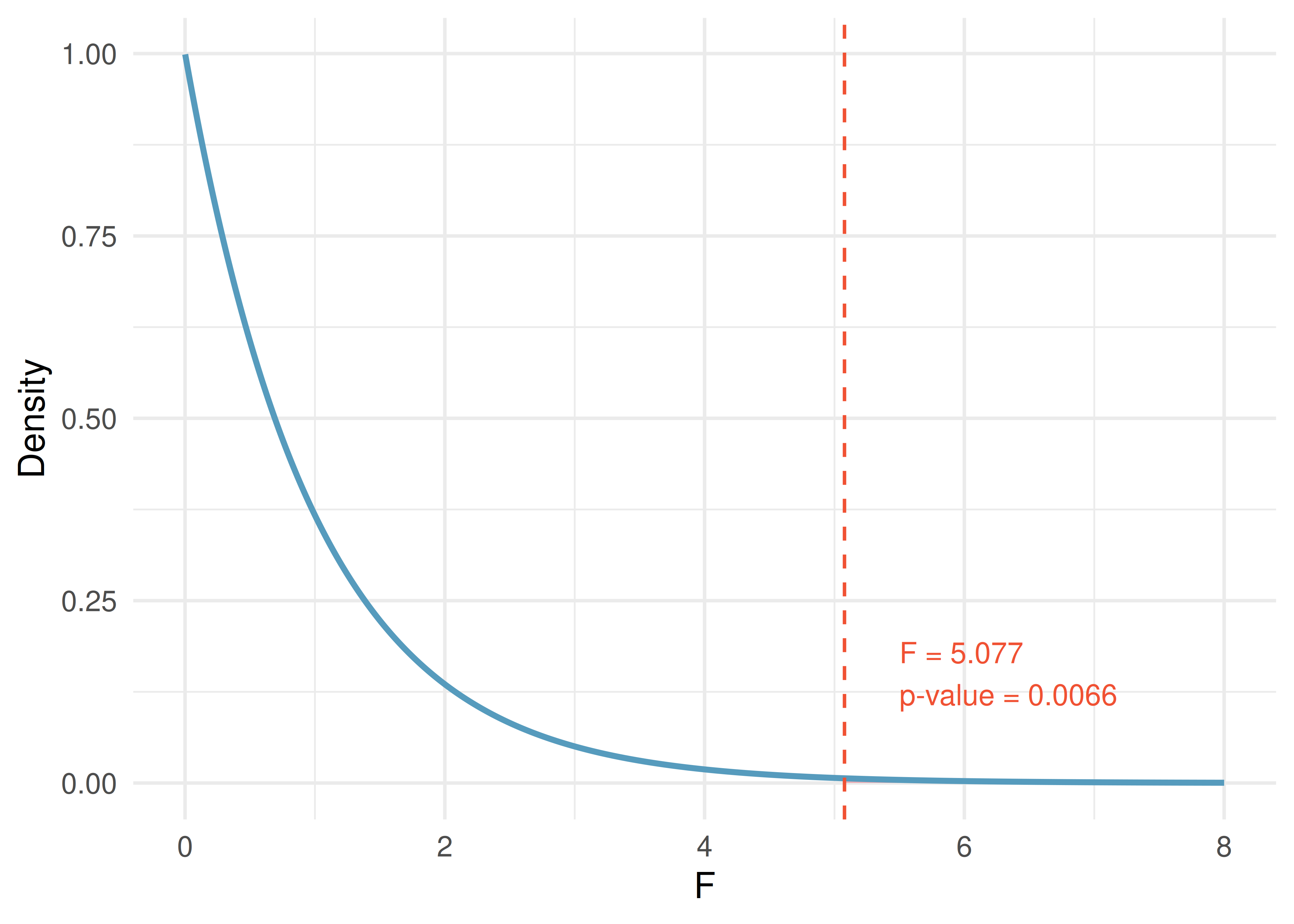
The p-value corresponding to \(F = 5.077\) with \(df_1 = 2\) and \(df_2 = 426\) is approximately 0.0066. Does this provide strong evidence against the null hypothesis?

---

The p-value is smaller than 0.05, indicating the evidence is strong enough to reject the null hypothesis at a discernibility level of 0.05. The data provide strong evidence that the average on-base percentage varies by player’s primary field position.

Note that the small p-value tells us there is a notable difference somewhere, but ANOVA does not tell us which group is different. Follow-up analyses (discussed in the next chapter on multiple comparisons) are needed.

17.3.3 Reading an ANOVA table

ANOVA results are commonly presented in a table. Here is the ANOVA table for the MLB data:

Source	df	Sum Sq	Mean Sq	F value	p-value
position	2	0.0161	0.00803	5.077	0.0066
Residuals	426	0.6740	0.00158

The key information is in the last two columns: the F-statistic (5.077) and the p-value (0.0066).

Components of an ANOVA table.

• Sum of Squares Between Groups (SSG): Measures the total variability of the group means around the overall mean. \(SSG = \sum_{j=1}^{k} n_j (\bar{x}_j - \bar{x})^2\).
• Sum of Squared Errors (SSE): Measures the total variability of observations around their group means. \(SSE = \sum_{j=1}^{k} (n_j - 1) s_j^2\).
• Sum of Squares Total (SST): The total variability in all observations. \(SST = SSG + SSE\).
• Mean Square Between Groups (MSG): \(MSG = SSG / (k - 1)\).
• Mean Square Error (MSE): \(MSE = SSE / (n - k)\).
• F-statistic: \(F = MSG / MSE\).

See it in action. Open the ANOVA omnibus walkthrough for a guided pass through framing → conditions → running the \(F\) → the “at least one differs” caveat. Or open the One-Way ANOVA tool or Randomization ANOVA directly. For post-hoc pairwise comparisons, append ?posthoc=tukey (or bonferroni) — see Ch 18.

17.4 Conditions for ANOVA

There are three conditions to check before performing ANOVA:

• Independence. If the data are a simple random sample, this condition is generally satisfied. For experiments, carefully consider whether the data may be independent (e.g., no pairing).

• Approximately normal. As with one- and two-sample testing for means, the normality assumption is especially important when sample sizes are small. With large sample sizes within each group, we look mainly for extreme outliers.

• Constant variance. The variability in the groups should be about equal. This can be checked by examining side-by-side box plots or comparing the standard deviations across groups. A common rule of thumb is that the ratio of the largest to smallest group standard deviation should be less than 2.

Figure 17.8: Histograms of OBP for each field position, showing that the distributions are reasonably bell-shaped and symmetric.

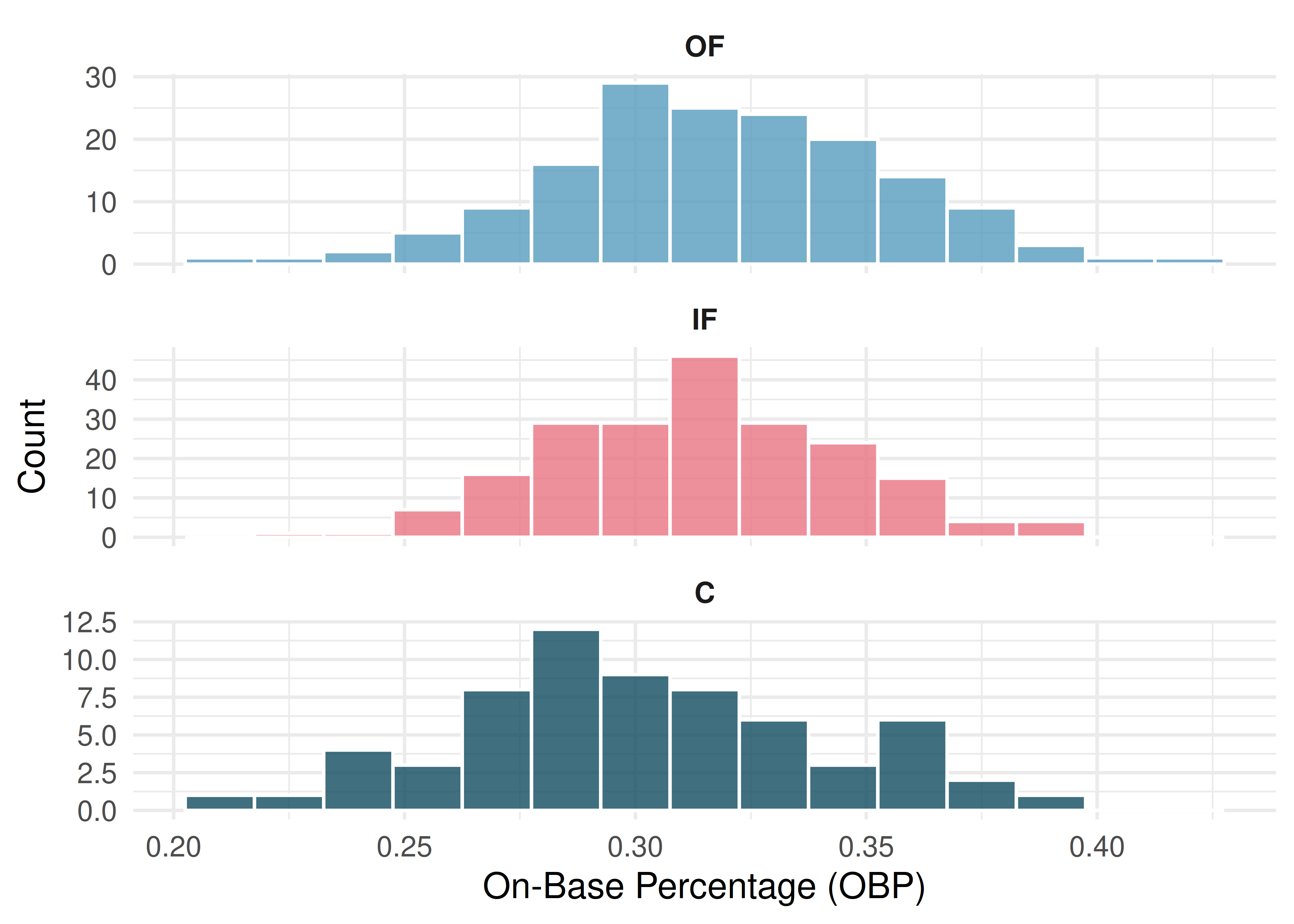
Diagnostics for an ANOVA analysis.

Independence is always important. The normality condition matters most when group sizes are small (with large groups, look only for extreme outliers). The constant variance condition is especially important when group sizes differ.

17.5 Chapter review

17.5.1 Summary

In this chapter, we introduced both the randomization test and the mathematical model for comparing means across two or more groups using ANOVA. The F-statistic measures the ratio of between-group variability (MSG) to within-group variability (MSE). When the null hypothesis is true and the conditions are satisfied, the F-statistic follows an F-distribution. A discernible result tells us that at least one group mean differs from the others, but does not identify which groups differ. For that, we need multiple comparison procedures — Bonferroni-adjusted pairwise CIs, Tukey’s HSD, and related methods — covered in the multiple comparisons chapter.

17.5.2 Key terms

• ANOVA (analysis of variance)
• F-statistic
• F-distribution
• F-test
• Mean square between groups (MSG)
• Mean square error (MSE)
• Sum of squares between groups (SSG)
• Sum of squared errors (SSE)
• Sum of squares total (SST)
• Degrees of freedom (ANOVA)
• Data snooping / data fishing

17.6 Exercises

Answers to odd-numbered exercises are provided in the Exercise Solutions appendix at the back of the book.

1. Fill in the blank. When doing an ANOVA, you observe large differences in means between groups. Within the ANOVA framework, this would most likely be interpreted as evidence strongly favoring the _____________ hypothesis.

2. Which test? We would like to test if students who are in the social sciences, natural sciences, arts and humanities, and other fields spend the same amount of time, on average, studying for a course. What type of test should we use? Explain your reasoning.

3. Cuckoo bird egg lengths, randomize once. Cuckoo birds lay their eggs in other birds’ nests, making them known as brood parasites. One question relates to whether the size of the cuckoo egg differs depending on the species of the host bird. (Latter 1902) Consider the following plots, one represents the original data, the second represents data where the host species has been randomly assigned to the egg length.

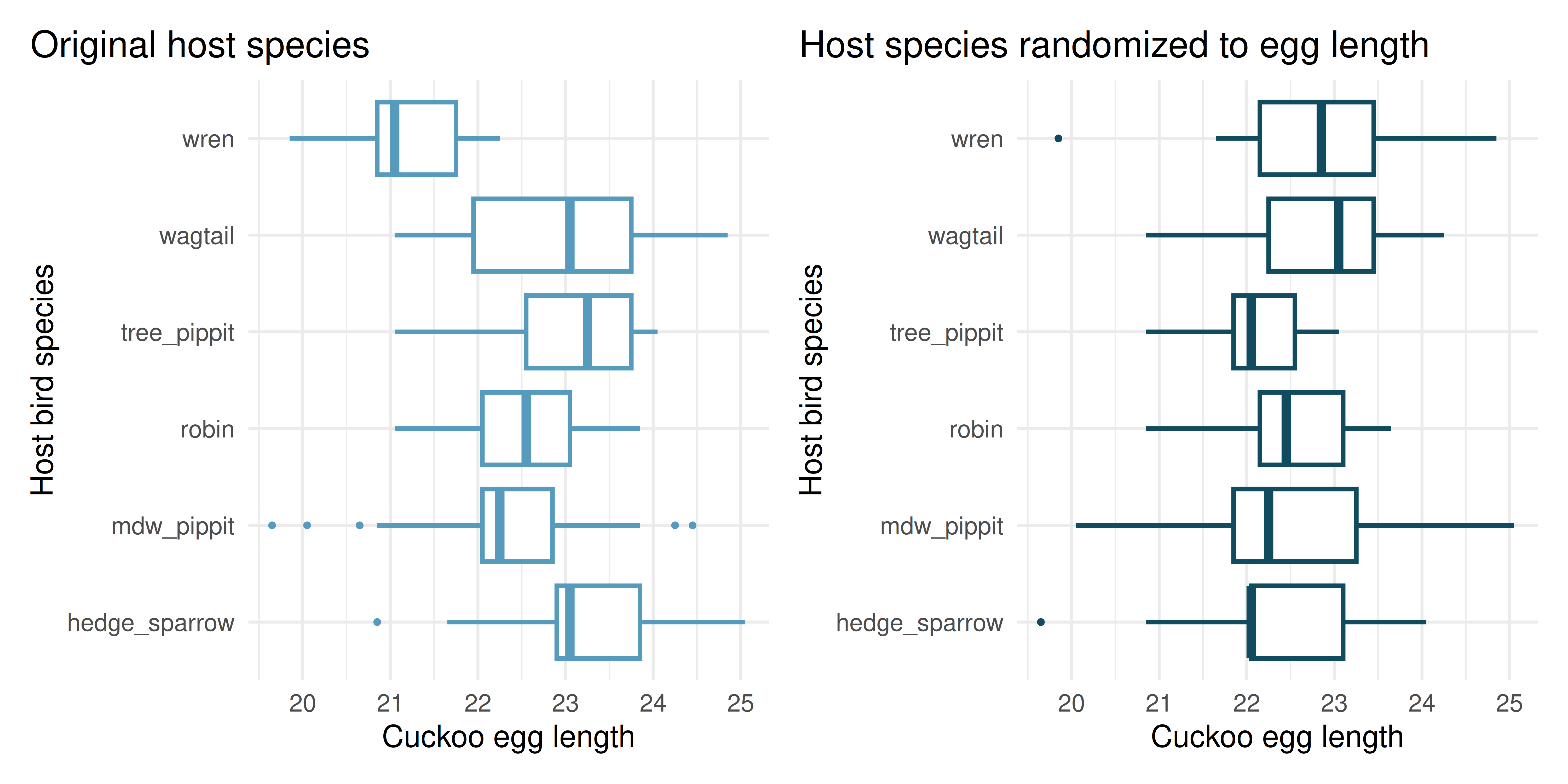
1. Consider the average length of the eggs for each species. Is the average length for the original data: more variable, less variable, or about the same as the randomized species? Describe what you see in the plots.

2. Consider the standard deviation of the lengths of the eggs within each species. Is the within species standard deviation of the length for the original data: bigger, smaller, or about the same as the randomized species?

3. Recall that the F statistic’s numerator measures how much the groups vary (MSG) with the denominator measuring how much the within species values vary (MSE), which of the plots above would have a larger F statistic, the original data or the randomized data? Explain.

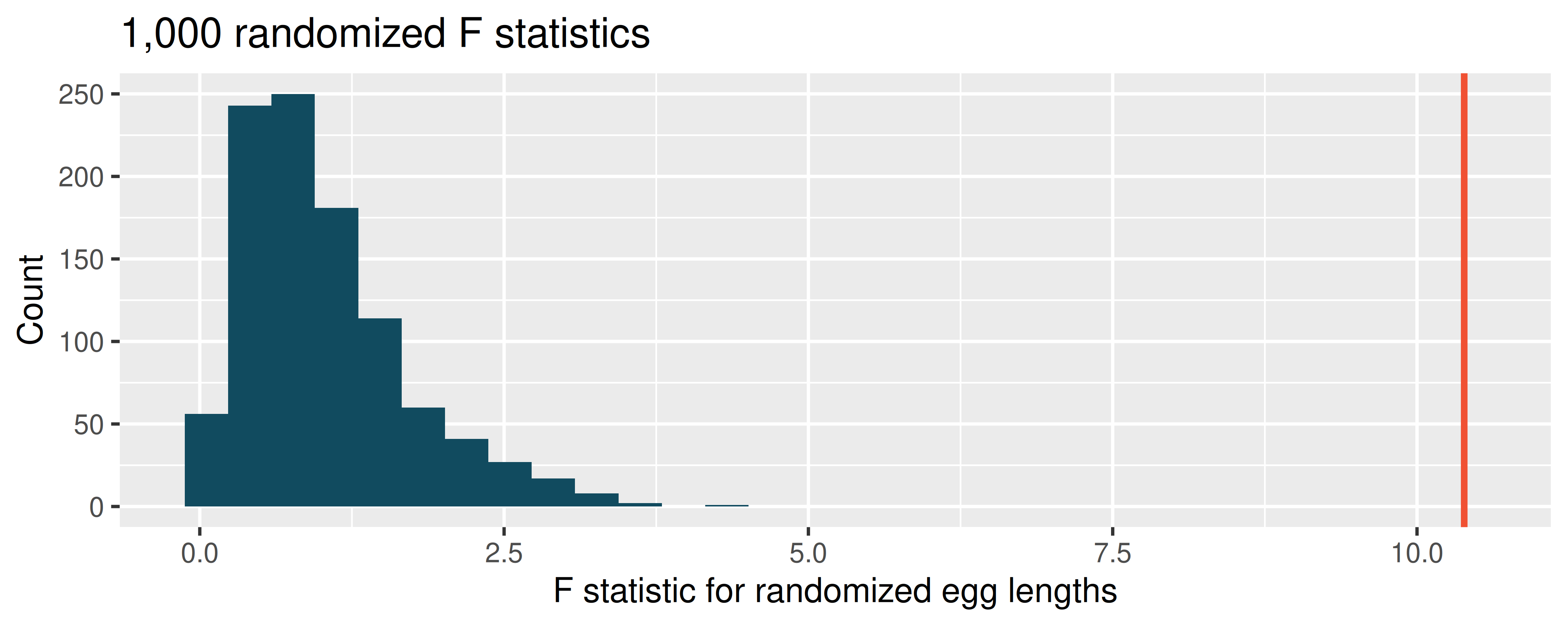
4. Cuckoo bird egg lengths, randomization test. Cuckoo birds lay their eggs in other birds’ nests, making them known as brood parasites. One question relates to whether the size of the cuckoo egg differs depending on the species of the host bird. (Latter 1902) Using the randomization distribution of the F statistic (host species randomized to egg length), conduct a hypothesis test to evaluate if there is a difference, in the population, between the average egg lengths for different host bird species. Make sure to state your hypotheses clearly and interpret your results in context of the data.

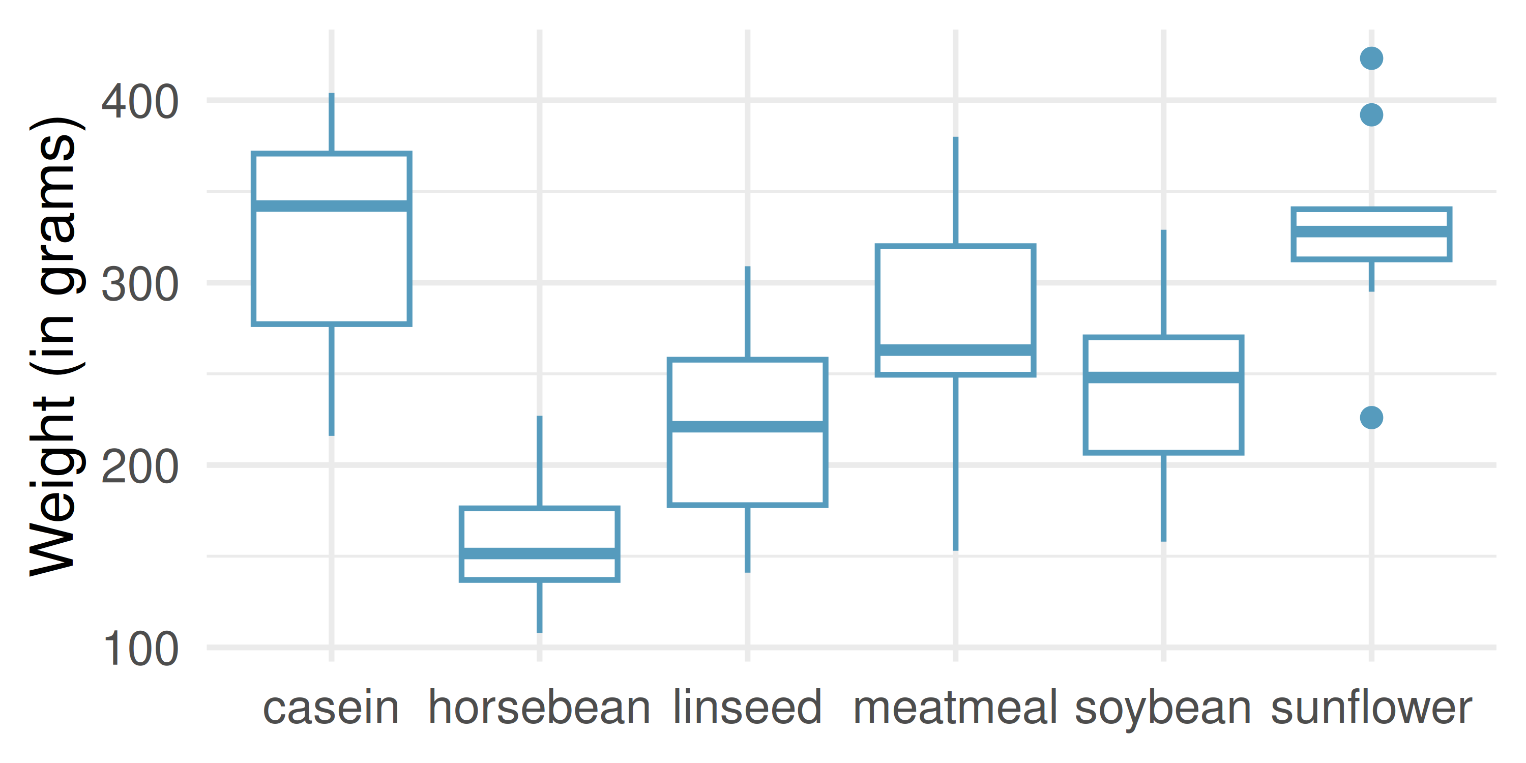
5. Chicken diet and weight, many groups. An experiment was conducted to measure and compare the effectiveness of various feed supplements on the growth rate of chickens. Newly hatched chicks were randomly allocated into six groups, and each group was given a different feed supplement. Sample statistics and a visualization of the observed data are shown below. (McNeil 1977)

Feed type	Mean	SD	n
casein	323.58	64.43	12
horsebean	160.20	38.63	10
linseed	218.75	52.24	12
meatmeal	276.91	64.90	11
soybean	246.43	54.13	14
sunflower	328.92	48.84	12

Using the ANOVA output below, conduct a hypothesis test to determine if these data provide convincing evidence that the average weight of chicks varies across some (or all) groups. Make sure to check relevant conditions.

term	df	sumsq	meansq	statistic	p.value
feed	5	231,129.2	46,225.832	15.3648	<0.0001
Residuals	65	195,556.0	3,008.554	NA	NA

6. Teaching descriptive statistics. A study compared five different methods for teaching descriptive statistics. The five methods were traditional lecture and discussion, programmed textbook instruction, programmed text with lectures, computer instruction, and computer instruction with lectures. 45 students were randomly assigned, 9 to each method. After completing the course, students took a 1-hour exam.

1. What are the hypotheses for evaluating if the average test scores are different for the different teaching methods?

2. What are the degrees of freedom associated with the \(F\)-test for evaluating these hypotheses?

3. Suppose the p-value for this test is 0.0168. What is the conclusion?

7. Coffee, depression, and physical activity. Caffeine is the world’s most widely used stimulant, with approximately 80% consumed in the form of coffee. Participants in a study investigating the relationship between coffee consumption and exercise were asked to report the number of hours they spent per week on moderate (e.g., brisk walking) and vigorous (e.g., strenuous sports and jogging) exercise. Based on these data the researchers estimated the total hours of metabolic equivalent tasks (MET) per week, a value always greater than 0. The table below gives summary statistics of MET for women in this study based on the amount of coffee consumed. (Lucas et al. 2011)

	Caffeinated coffee consumption
	1 cup / week or fewer	2-6 cups / week	1 cups / day	2-3 cups / day	4 cups / day or more
Mean	18.7	19.6	19.3	18.9	17.5
SD	21.1	25.5	22.5	22.0	22.0
n	12,215.0	6,617.0	17,234.0	12,290.0	2,383.0

1. Write the hypotheses for evaluating if the average physical activity level varies among the different levels of coffee consumption.

2. Check conditions and describe any assumptions you must make to proceed with the test.

3. Below is the output associated with this test. What is the conclusion of the test?

	df	sumsq	meansq	statistic	p.value
cofee	4	10,508	2,627	5.2	3e-04
Residuals	50,734	25,564,819	504	NA	NA
Total	50,738	25,575,327	NA	NA	NA

8. Student performance across discussion sections. A professor who teaches a large introductory statistics class (197 students) with eight discussion sections would like to test if student performance differs by discussion section, where each discussion section has a different teaching assistant. The summary table below shows the average final exam score for each discussion section as well as the standard deviation of scores and the number of students in each section.

	Sec 1	Sec 2	Sec 3	Sec 4	Sec 5	Sec 6	Sec 7	Sec 8
Mean	92.94	91.11	91.80	92.45	89.30	88.30	90.12	93.35
SD	4.21	5.58	3.43	5.92	9.32	7.27	6.93	4.57
n	33.00	19.00	10.00	29.00	33.00	10.00	32.00	31.00

The ANOVA output below can be used to test for differences between the average scores from the different discussion sections.

	df	sumsq	meansq	statistic	p.value
section	7	525.01	75.00	1.87	0.0767
Residuals	189	7,584.11	40.13	NA	NA
Total	196	8,109.12	NA	NA	NA

Conduct a hypothesis test to determine if these data provide convincing evidence that the average score varies across some (or all) groups. Check conditions and describe any assumptions you must make to proceed with the test.

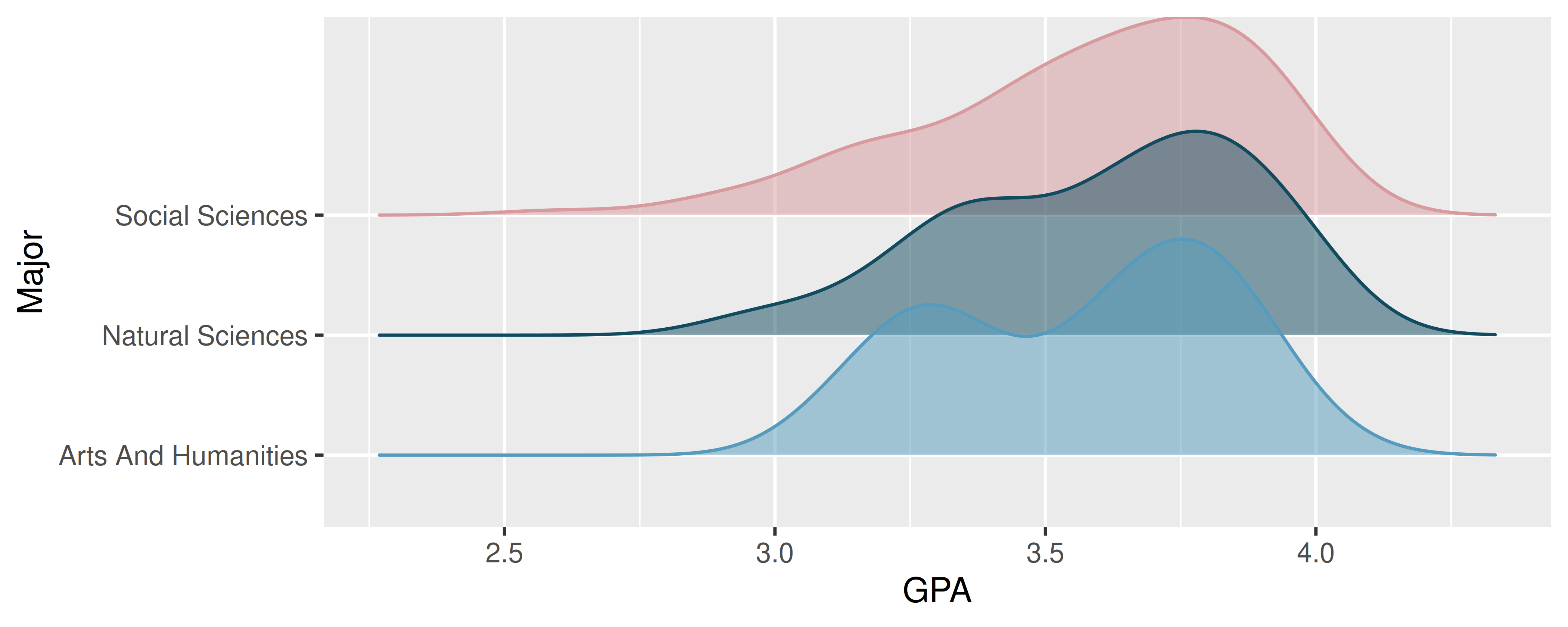
9. GPA and major. Undergraduate students in an introductory statistics course at Duke University conducted a survey about GPA and major. The density plots show the distributions of GPA among three groups of majors. ANOVA output is also provided.

term	df	sumsq	meansq	statistic	p.value
major	2	0.03	0.02	0.21	0.81
Residuals	195	15.77	0.08	NA	NA

1. Write the hypotheses for testing for a difference between average GPA across majors.

2. What is the conclusion of the hypothesis test?

3. How many students answered the questions on the survey, i.e., what is the sample size?

10. Work hours and education. The General Social Survey collects data on demographics, education, and work, among many other characteristics of US residents. (NORC 2010) Using ANOVA, we can consider educational attainment levels for all 1,172 respondents at once. Below are the distributions of hours worked by educational attainment and relevant summary statistics that will be helpful in carrying out this analysis.

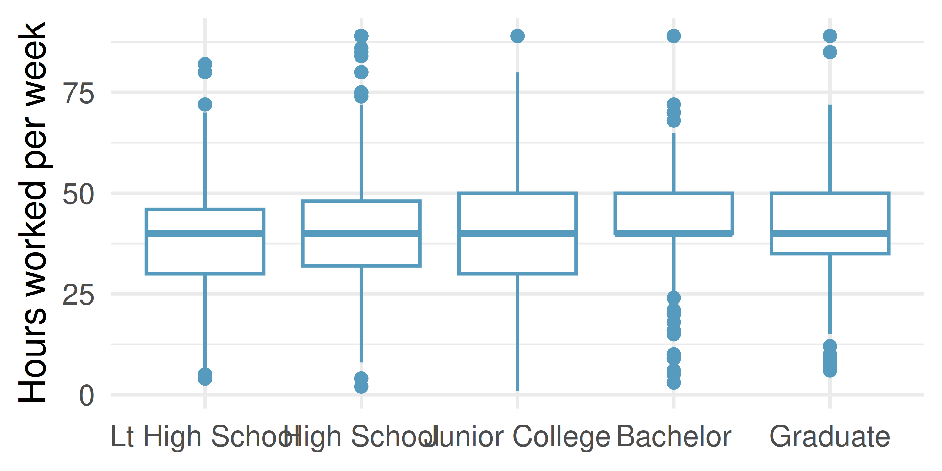
Educational attainment	Mean	SD	n
Lt High School	38.7	15.8	121
High School	39.6	15.0	546
Junior College	41.4	18.1	97
Bachelor	42.5	13.6	253
Graduate	40.8	15.5	155

1. Write hypotheses for evaluating whether the average number of hours worked varies across the five groups.

2. Check conditions and describe any assumptions you must make to proceed with the test.

3. Below is the output associated with this test. What is the conclusion of the test?

term	df	sumsq	meansq	statistic	p.value
degree	4	2,006.16	501.54	2.19	0.07
Residuals	1,167	267,382.16	229.12	NA	NA

11. Matching observed data with randomized F statistics. Consider the following two datasets. The response variable is the score and the explanatory variable is whether the individual is in one of four groups.

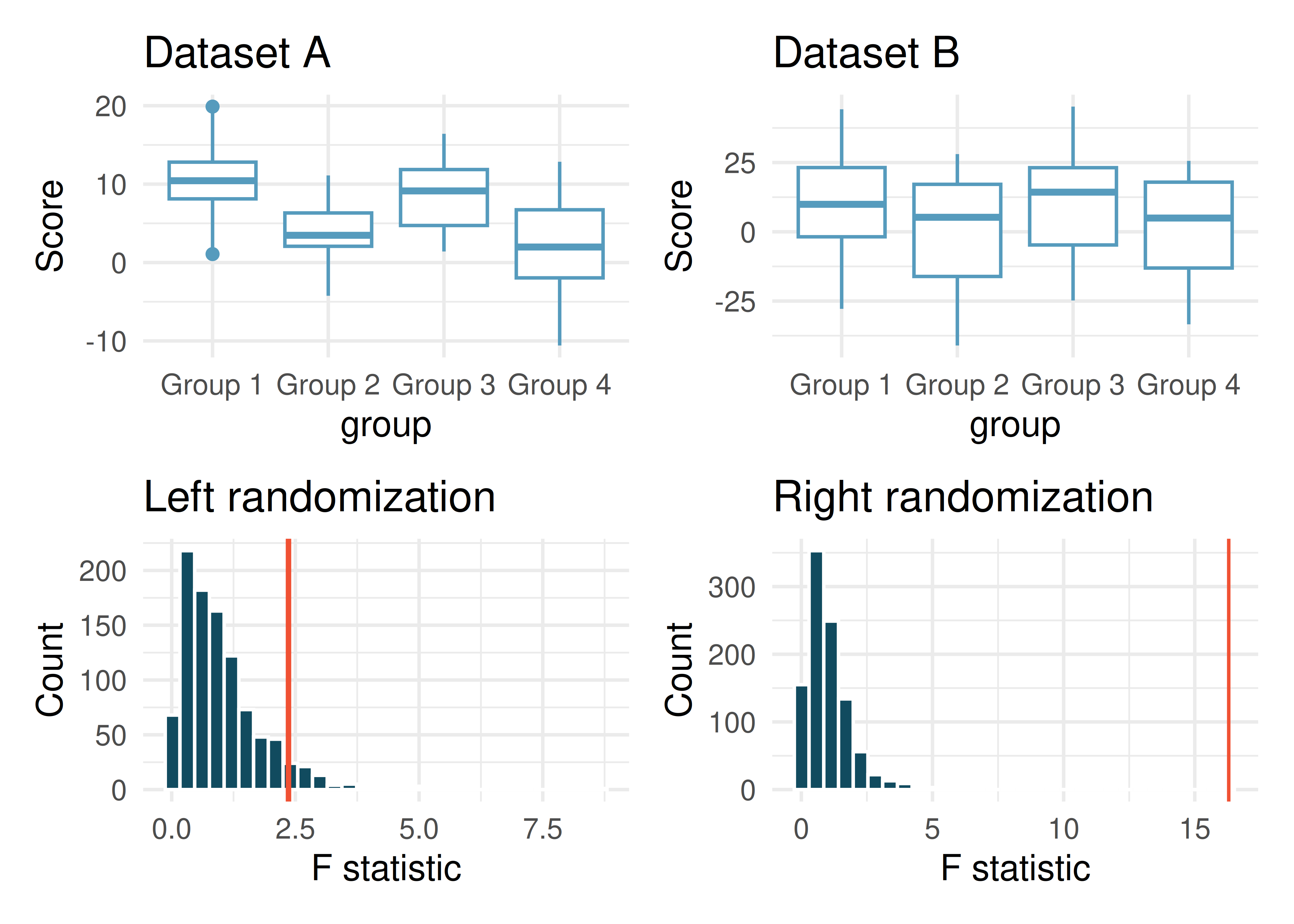
The randomizations (randomly assigning group to the score, calculating a randomization F statistic) were done 1000 times for each of Dataset A and B. The red line on each plot indicates the observed F statistic for the original (unrandomized) data.

1. Does the randomization distribution on the left correspond to Dataset A or B? Explain.

2. Does the randomization distribution on the right correspond to Dataset A or B? Explain.

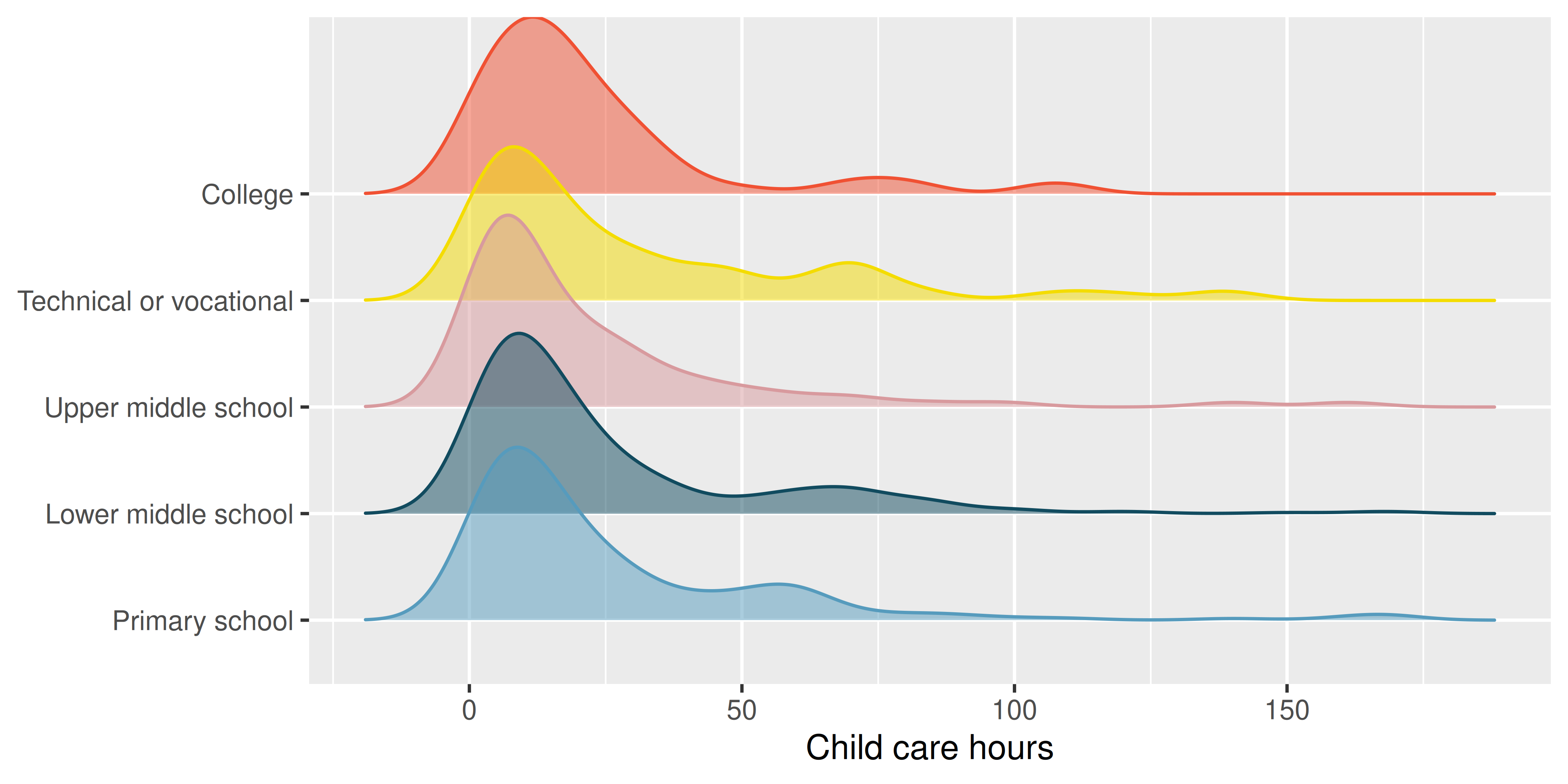
12. Child care hours. The China Health and Nutrition Survey aims to examine the effects of the health, nutrition, and family planning policies and programs implemented by national and local governments. (UNC Carolina Population Center 2006) It, for example, collects information on number of hours Chinese parents spend taking care of their children under age 6. The side-by-side box plots below show the distribution of this variable by educational attainment of the parent. Also provided below is the ANOVA output for comparing average hours across educational attainment categories.

term	df	sumsq	meansq	statistic	p.value
edu	4	4,142.09	1,035.52	1.26	0.28
Residuals	794	653,047.83	822.48	NA	NA

1. Write the hypotheses for testing for a difference between the average number of hours spent on child care across educational attainment levels.

2. What is the conclusion of the hypothesis test?

13. After a significant ANOVA, then what? A one-way ANOVA compares mean commute times across 4 city types (rural, suburban, small-city, big-city) using data from \(n = 200\) commuters. The ANOVA rejects \(H_0\): all population means are equal (\(F = 8.4\), p-value \(= 0.00003\)).

1. What does the significant \(F\)-test tell you? What does it not tell you?

2. A colleague suggests building all \(\binom{4}{2} = 6\) pairwise 95% CIs for the differences in means (rural − suburban, rural − small-city, rural − big-city, suburban − small-city, suburban − big-city, small-city − big-city). If each CI is constructed at the 95% confidence level, will the joint coverage — the probability that all six CIs simultaneously capture their true differences — be 95%? Above 95%? Below 95%? Explain in one sentence.

3. Name one method (from Ch 19 in this textbook, or from other courses) that adjusts pairwise CIs so that the joint coverage stays at (or above) 95%.

4. Why do we care about joint coverage rather than just individual coverage?

Dataset sources

Cuckoo (Stat2Data)

StatLens Exercises

Let StatLens do the arithmetic; spend your effort on the reasoning a calculator can’t do.

1. Frame the question. An agronomist randomly assigns plots to one of four fertilizer brands and measures yield (bushels/acre) at harvest. She has 30 plots per brand.

   1. Identify the explanatory variable, its number of levels, and the response.
   2. Write \(H_0\) and \(H_A\) for the omnibus ANOVA \(F\)-test in symbols and in words.
   3. Why does ANOVA use an \(F\)-statistic that compares two variances, when the question is really about means?

2. Choose the procedure. For each scenario, name the procedure — one-way ANOVA \(F\)-test, two-sample \(t\)-test, paired \(t\)-test, or not an ANOVA problem.

   1. Compare mean test scores across three teaching methods (random assignment).
   2. Compare mean test scores between two teaching methods (random assignment).
   3. Compare the proportion of students passing across four schools.
   4. Compare yields across four fertilizer brands, where the same plots received different brands in different years (within-plot pairing).
   5. Compare the mean grade of every student in three sections of the same course.

3. Check the conditions. Open the One-Way ANOVA tool with any multi-group numeric dataset.

   1. Name the three ANOVA conditions and state each in plain language.
   2. Inspect the side-by-side boxplots in StatLens. What pattern would convince you the equal-variance condition has failed?
   3. Suppose one group has \(n_1 = 8\) with a strong right skew, while two other groups have \(n_2 = n_3 = 50\) and look symmetric. Is ANOVA’s \(F\)-test trustworthy here? What’s a defensible alternative?

4. Run it and interpret it. Open the One-Way ANOVA tool with any multi-group numeric dataset.

   1. Report the \(F\)-statistic, the two df values (between and within), and the p-value.

   2. State your decision at \(\alpha = 0.05\) and write a one-sentence conclusion in context.

   3. Suppose \(F\) is large and the p-value is 0.002. The conclusion “the four groups all have different means” is wrong. Why? What is the correct conclusion?

   4. Which statement is the correct interpretation of \(F = 4.5\)?

      1. Group means differ by an average of 4.5 units.
      2. The between-group variance is 4.5 times the within-group variance, in this sample.
      3. About 4.5% of the variability is explained by the group factor.

5. Simulation as a sanity check. Open the Randomization ANOVA on the same data.

   1. Run 5000 simulated \(F\) statistics under \(H_0\) (group labels shuffled). What does the null distribution look like? Is it \(F\)-shaped?
   2. Compare the simulation p-value to the \(F\)-distribution p-value from Exercise 4. How close are they?
   3. Repeat on a dataset where one group has only \(n = 6\) observations with a clear outlier. Are the two p-values still close? Which is the safer one to report?
   4. A student says: “If I’m going to run the randomization version anyway, why learn the \(F\)-distribution?” Give two good reasons. (Hint: think about understanding the \(F\) statistic, and speed for routine reporting.)

Latter, O. H. 1902. “The Egg of Cuculus Canorus. An Enquiry into the Dimensions of the Cuckoo’s Egg and the Relation of the Variations to the Size of the Eggs of the Foster-Parent, with Notes on Coloration.” Biometrika 1: 164–76. https://doi.org/10.2307/2331486.

Lucas, M., F. Mirzaei, A. Pan, O. I. Okereke, W. C. Willett, E. J. O’Reilly, K. Koenen, and A. Ascherio. 2011. “Coffee, Caffeine, and Risk of Depression Among Women.” Archives of Internal Medicine 171 (17): 1571. https://doi.org/10.1001/archinternmed.2011.393.

McNeil, D. R. 1977. “Interactive Data Analysis: A Practical Primer.”

NORC. 2010. http://www.openintro.org/redirect.php?go=textbook-gss_2010.

UNC Carolina Population Center. 2006. “China Health and Nutrition Survey, 2006.” http://www.openintro.org/redirect.php?go=textbook-china_health_nut_survey_2006.