Project: Exploring a Distribution

Project — Exploratory Data Analysis. A project is a short analysis you carry out end to end and communicate as a brief report. Do the work in Jamovi (or R) and submit the deliverable described at the end. The skill here is producing the right summaries and reading them honestly.

The question

Collectors buy and sell the game Mario Kart (Nintendo Wii) in online auctions. You have the final prices from a sample of completed auctions.

What is a typical selling price, how much do prices vary, and do new and used copies sell differently?

The data

The mariokart dataset holds 143 eBay auctions. You’ll use total_pr (final price, in dollars) and cond (new or used). A couple of auctions were bundles sold at unusually high prices — keep an eye out for outliers.

Plan it first

1. Variable types. Classify total_pr and cond.
2. Displays & summaries. To describe one numerical variable, which display and which numerical summaries are appropriate?
3. Resistance. Given the possible high-price outliers, which measures of center and spread will you trust — mean/SD or median/IQR — and why?
4. Comparison. To compare price for new vs. used, which display fits a numerical variable split by a categorical one?

Do the analysis

Jamovi

1. Open mariokart.csv (Open → Data).
2. Exploration → Descriptives. Put total_pr in Variables and cond in Split by. Request mean, median, std. deviation, IQR.
3. Under Plots, turn on a histogram and a box plot.
4. Read off the typical price, the spread, and how new vs. used compare.

(Jamovi screenshots to be added.)

R

library(dplyr)
library(ggplot2)
library(patchwork)
library(openintro)
data(mariokart)

# Overall numerical summary (note how outliers pull the mean above the median)
mariokart |>
  summarize(mean = mean(total_pr), median = median(total_pr),
            sd = sd(total_pr), IQR = IQR(total_pr))

# A tibble: 1 × 4
   mean median    sd   IQR
  <dbl>  <dbl> <dbl> <dbl>
1  49.9   46.5  25.7  12.8

# Center & spread by condition (median/IQR are resistant to the outliers)
mariokart |>
  group_by(cond) |>
  summarize(median = median(total_pr), IQR = IQR(total_pr), n = n())

# A tibble: 2 × 4
  cond  median   IQR     n
  <fct>  <dbl> <dbl> <int>
1 new     54.0  9.75    59
2 used    42.8  8.91    84

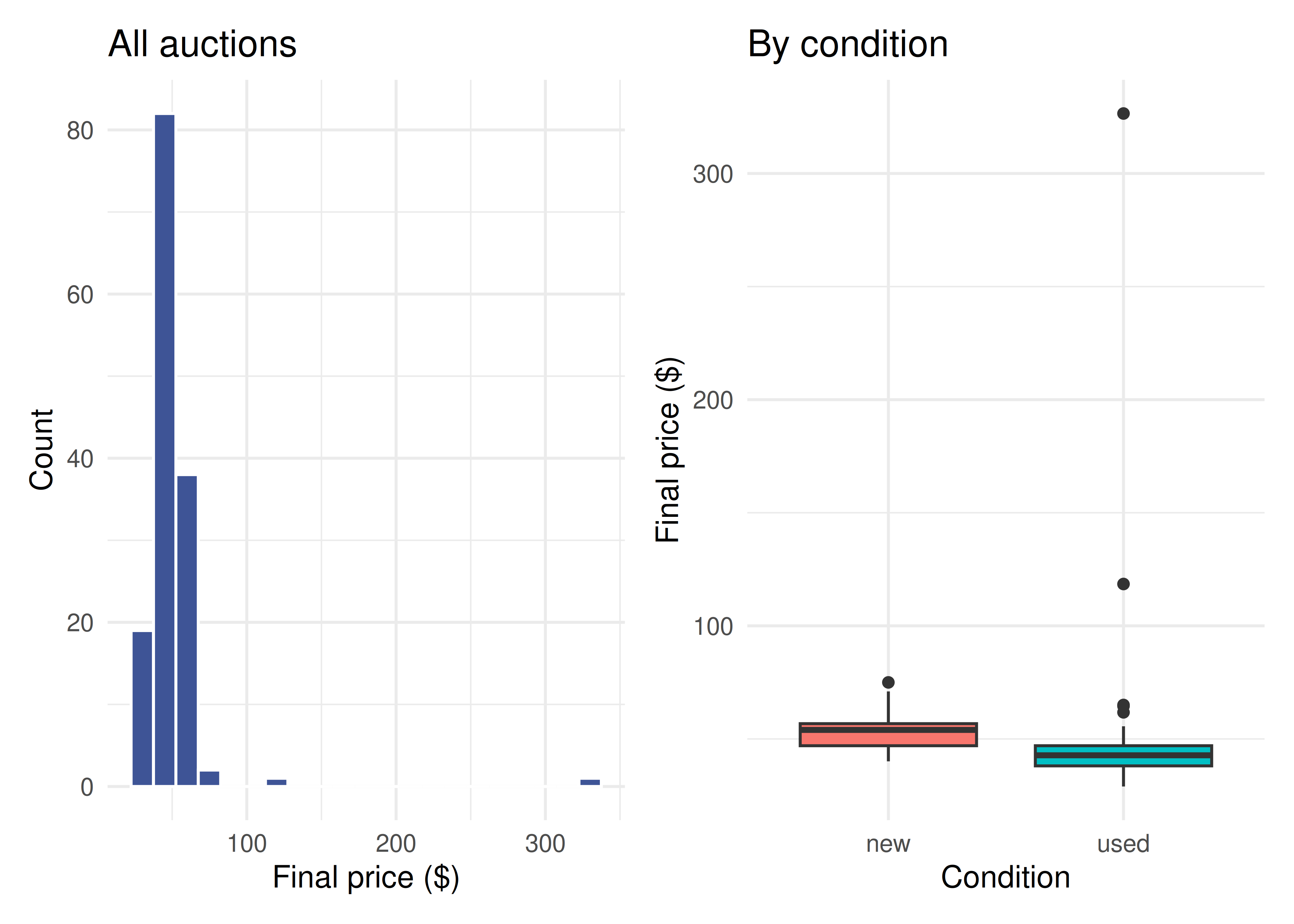
p1 <- ggplot(mariokart, aes(total_pr)) +
  geom_histogram(binwidth = 15, fill = "#3E5496", color = "white") +
  labs(x = "Final price ($)", y = "Count", title = "All auctions") +
  theme_minimal(base_size = 12)

p2 <- ggplot(mariokart, aes(cond, total_pr, fill = cond)) +
  geom_boxplot(show.legend = FALSE) +
  labs(x = "Condition", y = "Final price ($)", title = "By condition") +
  theme_minimal(base_size = 12)

p1 + p2

Distribution of Mario Kart auction prices (left) and prices split by condition (right). A couple of high-priced bundle auctions stretch the right tail.

Your deliverable

Submit a short report containing all of:

1. Graphic — a labeled histogram of total_pr (and, for the comparison, side-by-side boxplots by cond).
2. Center & spread — report the median and IQR, and say why you chose them over the mean and SD here.
3. Shape & outliers — describe the shape (symmetric? skewed?) and identify any outliers, with a sentence on what they are.
4. Comparison in context — 2–3 sentences comparing new vs. used prices.
5. One limitation — e.g., these are only completed auctions of one game on one platform.

How it’s graded

Criterion	What we look for
Appropriate, labeled graphic	histogram + boxplots, axes labeled
Right summaries for the data	median/IQR chosen given the outliers, justified
Shape & outliers described	correct shape; outliers identified
Comparison in context	new vs. used stated in plain language
Communication	clear, correct, no over-claiming

Warm up first. Explore the same kind of summaries interactively in the Descriptive Statistics explorer before building your report.