25 Random Variables
In the previous chapter, we developed rules for computing probabilities of events. Now we shift our focus to random variables — numerical summaries of random processes. A random variable assigns a number to each outcome of a random process, which allows us to apply mathematical tools for prediction and analysis. We distinguish between discrete and continuous random variables, introduce probability distributions, and build the foundation for the specific distributions (binomial and normal) that follow in later chapters.
25.1 Random variables
It is often useful to model a random process by assigning a number to each outcome. This numerical model is called a random variable.
A random variable is a numerical outcome of a random process. We typically denote random variables with capital letters such as \(X\), \(Y\), or \(Z\), and their observed values with the corresponding lowercase letters \(x\), \(y\), or \(z\).
Two books are assigned for a statistics class: a textbook ($137) and a study guide ($33). The university bookstore has determined that 20% of enrolled students buy neither book, 55% buy the textbook only, and 25% buy both books. If \(X\) represents the amount a single student spends on books, then \(X\) is a random variable with possible values $0, $137, and $170.
Random variables come in two types — discrete and continuous — and the distinction matters because they require different mathematical tools.
25.2 Discrete random variables
A discrete random variable takes on a finite or countably infinite number of distinct values. These values can be listed (even if the list is infinitely long).
Examples of discrete random variables:
- The number showing when you roll a die: \(X \in \{1, 2, 3, 4, 5, 6\}\)
- The number of heads in 10 coin flips: \(X \in \{0, 1, 2, \ldots, 10\}\)
- The number of customers arriving at a store in an hour: \(X \in \{0, 1, 2, 3, \ldots\}\)
25.2.1 Why the distinction matters
In Parts II and III, we worked extensively with sample statistics like the sample mean \(\bar{x}\) and the sample proportion \(\hat{p}\). These are actually observed values of random variables. The sampling distribution of \(\bar{x}\) that we studied in the sampling distributions chapter is really the probability distribution of a random variable. Formalizing the language of random variables helps us state results more precisely and connect our earlier simulation-based reasoning to mathematical theory.
25.2.2 Probability mass functions
The complete description of a discrete random variable is given by its probability mass function (PMF), which specifies the probability of each possible value.
The probability mass function (PMF) of a discrete random variable \(X\) is the function \(P(X = x)\) that gives the probability that \(X\) takes on each possible value \(x\). A valid PMF must satisfy:
- \(P(X = x) \geq 0\) for every value \(x\).
- The sum of all probabilities equals 1: \(\sum_{\text{all } x} P(X = x) = 1\).
The bookstore example from the previous section has the following PMF:
| \(x_i\) | $0 | $137 | $170 |
|---|---|---|---|
| \(P(X = x_i)\) | 0.20 | 0.55 | 0.25 |
We can verify this is a valid PMF: all probabilities are between 0 and 1, and \(0.20 + 0.55 + 0.25 = 1.00\).
Suppose a campus shuttle arrives every 10 minutes. The number of students who board the shuttle at a particular stop can be modeled with the following distribution:
| Number of students (\(x\)) | 0 | 1 | 2 | 3 | 4 |
|---|---|---|---|---|---|
| \(P(X = x)\) | 0.10 | 0.25 | 0.35 | 0.20 | 0.10 |
- Verify this is a valid probability distribution. (b) What is the probability that 2 or fewer students board? (c) What is the probability that more than 2 students board?
Show answer
- All probabilities are between 0 and 1, and \(0.10 + 0.25 + 0.35 + 0.20 + 0.10 = 1.00\). (b) \(P(X \leq 2) = 0.10 + 0.25 + 0.35 = 0.70\). (c) \(P(X > 2) = 1 - P(X \leq 2) = 1 - 0.70 = 0.30\), or equivalently \(0.20 + 0.10 = 0.30\).
25.2.3 Visualizing discrete distributions
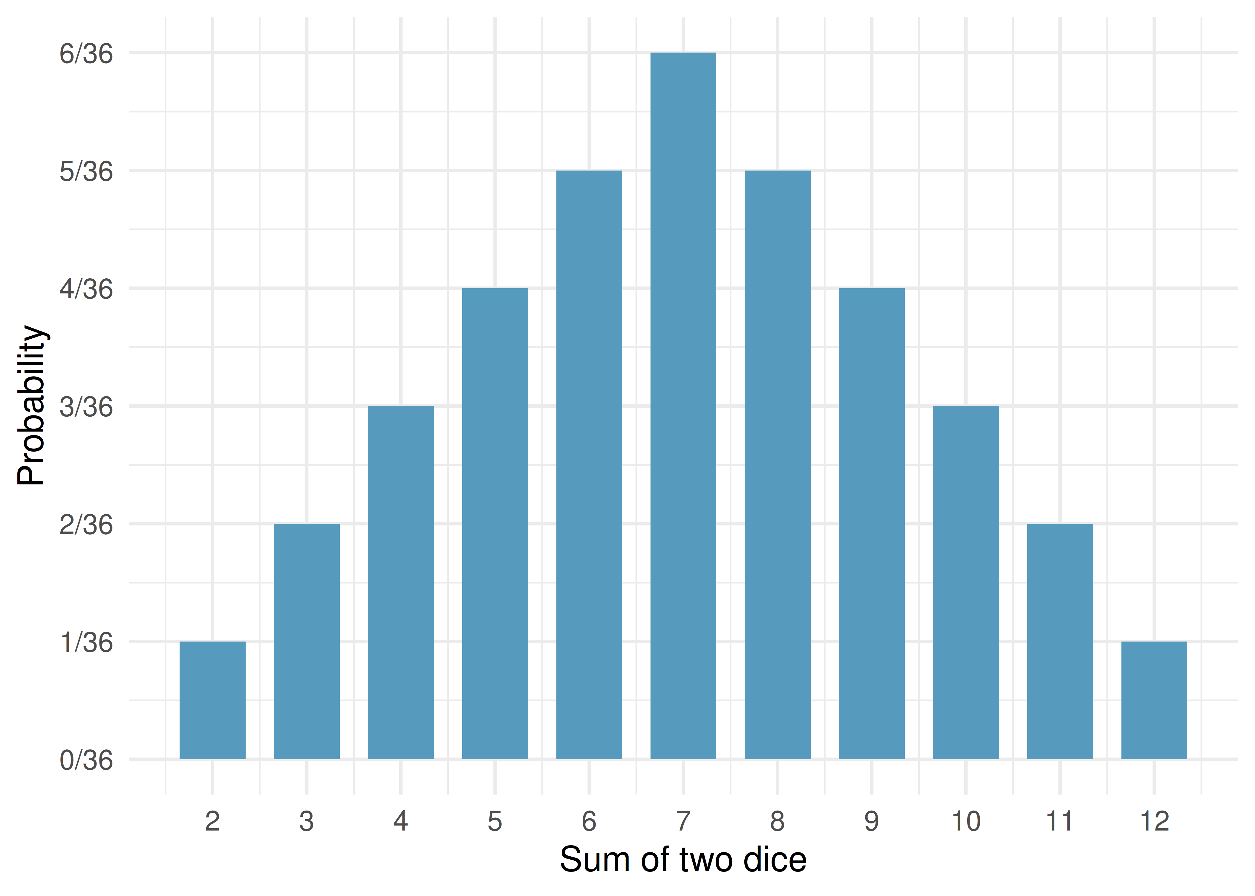
Discrete probability distributions are often displayed as bar plots where the height of each bar represents the probability of that outcome. When the outcomes are numerical, we place the bars at their numerical locations, creating a plot that resembles a histogram.
25.2.4 Building intuition with simulation
We can also estimate a probability distribution by simulating the random process many times and recording the relative frequencies of each outcome. For example, if we simulate rolling two dice 10,000 times and record the sum each time, the histogram of those 10,000 sums will closely approximate the theoretical probability distribution. As the number of simulations increases, the approximation improves — this is the Law of Large Numbers in action.
This connection between simulation and theory is one of the most important ideas in the course. Every time we used simulation in Parts II and III to build a null distribution or a bootstrap distribution, we were approximating a theoretical probability distribution.
25.3 Cumulative distribution functions
The cumulative distribution function (CDF) of a random variable \(X\) is the function:
\[F(x) = P(X \leq x)\]
The CDF gives the probability that \(X\) takes a value less than or equal to \(x\).
The CDF is a useful alternative to the PMF for answering “at most” or “at least” types of questions. For a discrete random variable, the CDF is a step function that jumps at each possible value of \(X\).
Consider the sum of two dice. The CDF at a few key values:
| \(x\) | 2 | 3 | 4 | 5 | 6 | 7 | 8 | 9 | 10 | 11 | 12 |
|---|---|---|---|---|---|---|---|---|---|---|---|
| \(F(x) = P(X \leq x)\) | \(\frac{1}{36}\) | \(\frac{3}{36}\) | \(\frac{6}{36}\) | \(\frac{10}{36}\) | \(\frac{15}{36}\) | \(\frac{21}{36}\) | \(\frac{26}{36}\) | \(\frac{30}{36}\) | \(\frac{33}{36}\) | \(\frac{35}{36}\) | \(\frac{36}{36}\) |
Key properties of any CDF:
- \(F(x)\) is non-decreasing: if \(a < b\), then \(F(a) \leq F(b)\).
- \(F(x) \to 0\) as \(x \to -\infty\) and \(F(x) \to 1\) as \(x \to +\infty\).
- \(P(a < X \leq b) = F(b) - F(a)\).
The CDF becomes especially important for continuous random variables, where individual values have zero probability and we must always work with intervals.
Using the CDF for the sum of two dice above, find: (a) \(P(X \leq 5)\). (b) \(P(X > 9)\). (c) \(P(4 < X \leq 8)\).
Show answer
- \(F(5) = 10/36\). (b) \(P(X > 9) = 1 - F(9) = 1 - 30/36 = 6/36 = 1/6\). (c) \(P(4 < X \leq 8) = F(8) - F(4) = 26/36 - 6/36 = 20/36 = 5/9\).
25.4 Continuous random variables
A continuous random variable can take any value in some interval of real numbers. Its probability distribution is described by a smooth curve called a probability density function (PDF).
Examples of continuous random variables:
- The height of a randomly selected adult
- The time until the next bus arrives
- The temperature at noon tomorrow
25.4.1 From histograms to density curves
When we have a very large sample and use very narrow bins in a histogram, the outline of the histogram starts to look like a smooth curve. This smooth curve is a probability density function.
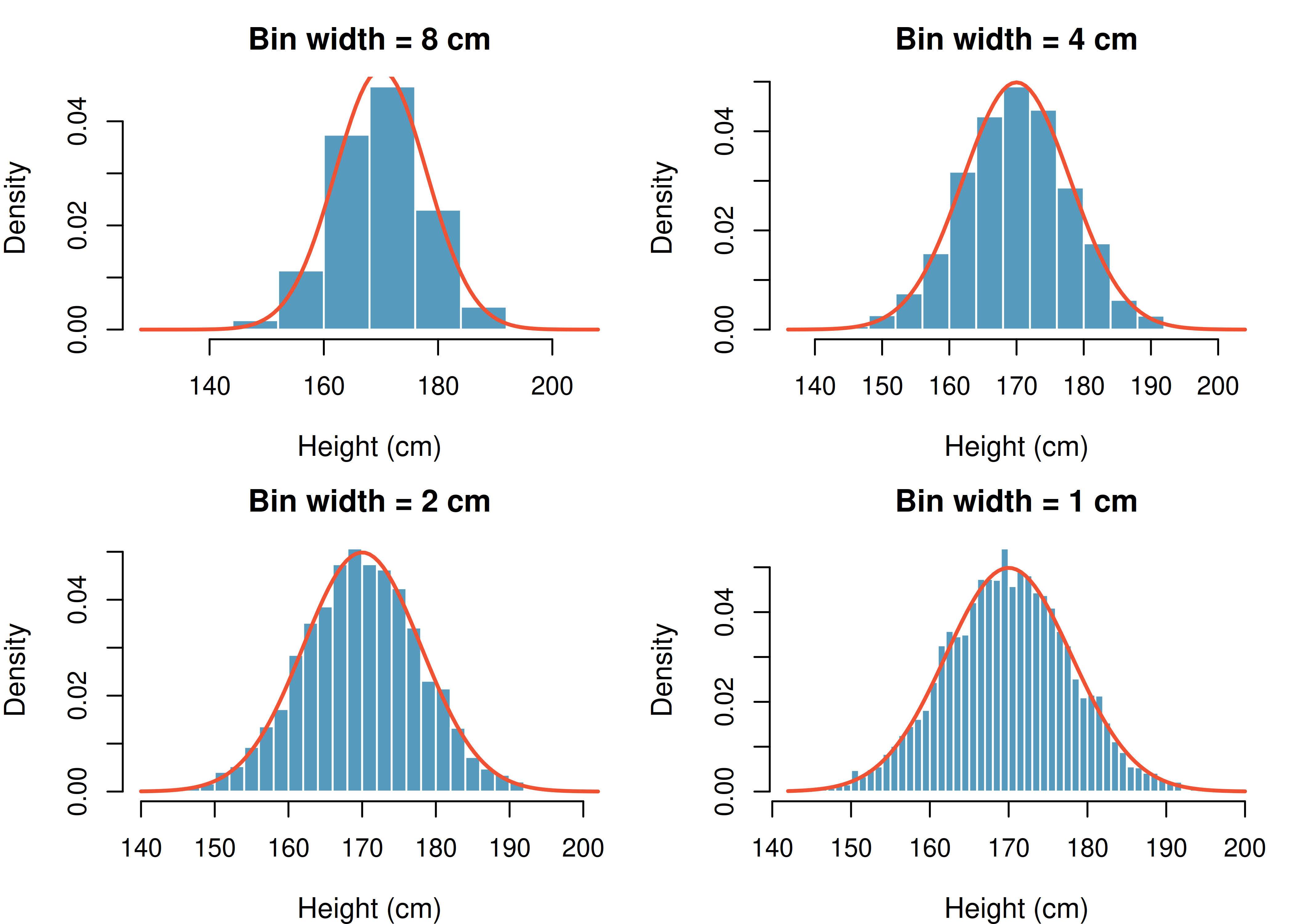
Properties of a probability density function (PDF):
- The density curve is always on or above the horizontal axis: \(f(x) \geq 0\) for all \(x\).
- The total area under the curve equals 1.
- The probability that \(X\) falls between \(a\) and \(b\) equals the area under the curve between \(a\) and \(b\): \(P(a \leq X \leq b) = \text{area between } a \text{ and } b\).
25.4.2 Probabilities from continuous distributions
For a continuous random variable, probabilities are areas under the density curve.
The heights of US adults follow a continuous distribution. What proportion of the population has heights between 180 cm and 185 cm?
Using the density curve, we find the area under the curve between 180 and 185:
\[P(180 \leq X \leq 185) = \text{area between 180 and 185} \approx 0.1157\]
About 11.6% of US adults are between 180 and 185 cm tall.
A key difference: the probability of an exact value is zero for continuous random variables.
For a continuous random variable, \(P(X = c) = 0\) for any specific value \(c\). There is no area under the curve at a single point. This means:
\[P(X \leq a) = P(X < a)\]
This is not true for discrete random variables, where individual outcomes carry positive probability.
If \(P(180 \leq \text{height} \leq 185) = 0.1157\) for a randomly selected US adult, and three adults are selected at random: (a) What is the probability all three have heights between 180 and 185 cm? (b) What is the probability none of them do?
Show answer
- Since the selections are independent: \(0.1157^3 \approx 0.0015\). (b) \((1 - 0.1157)^3 = 0.8843^3 \approx 0.692\).
25.4.3 Discrete vs. continuous: a summary
| Feature | Discrete | Continuous |
|---|---|---|
| Values | Finite or countable list | Any value in an interval |
| Described by | Probability mass function (PMF) | Probability density function (PDF) |
| \(P(X = c)\) | Can be positive | Always equals 0 |
| Probabilities | Sum probabilities of individual values | Find areas under the curve |
| Visualization | Bar plot | Smooth curve |
| Example | Number of coin flips until heads | Height of a randomly selected person |
In this course, we will work primarily with two specific distributions:
- The binomial distribution (the binomial distribution chapter) — a discrete distribution
- The normal distribution (the normal distribution chapter) — a continuous distribution
Understanding the general concepts from this chapter will make those specific distributions much easier to work with.
25.5 Chapter review
25.5.1 Summary
- A random variable assigns a numerical value to each outcome of a random process.
- Discrete random variables take on a finite or countable set of values. Their distributions are described by probability mass functions (PMFs).
- Continuous random variables can take any value in an interval. Their distributions are described by probability density functions (PDFs), and probabilities are calculated as areas under the curve.
- The cumulative distribution function (CDF) gives \(P(X \leq x)\) and works for both discrete and continuous random variables.
- For continuous random variables, \(P(X = c) = 0\) for any specific value \(c\).
- A valid probability distribution has non-negative probabilities that sum (or integrate) to 1.
25.6 Exercises
- College smokers. At a university, 13% of students smoke.
Calculate the expected number of smokers in a random sample of 100 students from this university.
The university gym opens at 9 am on Saturday mornings. One Saturday morning at 8:55 am there are 27 students outside the gym waiting for it to open. Should you use the same approach from part (a) to calculate the expected number of smokers among these 27 students?
- Carnival prize wheel. A carnival prize wheel has 10 equally-likely sectors: 5 say “Try Again” (win $0), 3 pay $3, 1 pays $10, and 1 pays a $25 jackpot. Let \(W\) be your winnings from one spin.
Compute \(E(W)\) and \(\text{SD}(W)\).
What is the maximum amount a risk-neutral player should be willing to pay per spin? Explain.
- Marble draws without replacement. A carnival booth has a bag of 12 marbles: 5 red, 4 blue, and 3 green. You draw 3 marbles without replacement. The payouts are $40 for 3 reds, $25 for 3 blues, and $0 for any other draw. Let \(W\) be your winnings.
Compute \(E(W)\) and \(\text{SD}(W)\).
The booth charges $5 to play. Let \(N = W - 5\) be your net profit on a single play. Compute \(E(N)\) and \(\text{SD}(N)\).
Based on \(E(N)\), should a risk-neutral player play this game? Explain.
- Is it worth it. Andy is always looking for ways to make money fast. Lately, he has been trying to make money by gambling. Here is the game he is considering playing: The game costs $2 to play. He draws a card from a deck. If he gets a number card (2-10), he wins nothing. For any face card ( jack, queen or king), he wins $3. For any ace, he wins $5, and he wins an extra $20 if he draws the ace of clubs.
Create a probability model and find Andy’s expected profit per game.
Would you recommend this game to Andy as a good way to make money? Explain.
- Cat weights. The histogram shown below represents the weights (in kg) of 47 female and 97 male cats.
What fraction of these cats weigh less than 2.5 kg?
What fraction of these cats weigh between 2.5 and 2.75 kg?
What fraction of these cats weigh between 2.75 and 3.5 kg?
- Income and gender. The relative frequency table below displays the distribution of annual total personal income (in 2009 inflation-adjusted dollars) for a representative sample of 96,420,486 Americans. These data come from the American Community Survey for 2005-2009. This sample is comprised of 59% males and 41% females.
Describe the distribution of total personal income.
What is the probability that a randomly chosen US resident makes less than $50,000 per year?
What is the probability that a randomly chosen US resident makes less than $50,000 per year and is female? Note any assumptions you make.
The same data source indicates that 71.8% of females make less than $50,000 per year. Use this value to determine whether or not the assumption you made in part (c) is valid.
{
| $10,000 to $14,999 | 4.7% |
|---|---|
| $15,000 to $24,999 | 15.8% |
| $25,000 to $34,999 | 18.3% |
| $35,000 to $49,999 | 21.2% |
| $50,000 to $64,999 | 13.9% |
| $65,000 to $74,999 | 5.8% |
| $75,000 to $99,999 | 8.4% |
| $100,000 or more | 9.7% |
}
- Grade distributions. Each row in the table below is a proposed grade distribution for a class. Identify each as a valid or invalid probability distribution, and explain your reasoning.
| Grades | |
|---|---|
| (b) | 0 |
| (c) | 0.3 |
| (d) | 0.3 |
| (e) | 0.2 |
| (f) | 0 |
- Three-round trivia bet. A trivia contestant has a 50% chance of answering any given question correctly, and questions are independent. She plays three rounds. Each round she places a $1 bet: a correct answer wins her $1, a wrong answer loses $1. Let \(Y\) be her total winnings after the three rounds.
The possible values of \(Y\) are \(-\$3, -\$1, +\$1, +\$3\). Compute the probability of each, and then compute \(E(Y)\).