7 Randomization Tests
Statistical inference is primarily concerned with understanding and quantifying the uncertainty of parameter estimates. While the equations and details change depending on the setting, the foundations for inference are the same throughout all of statistics. In this chapter, we introduce the hypothesis testing framework — a formal method for evaluating competing claims about a population using data. We learn how to build randomization distributions by shuffling data under the assumption that there is no effect, and we use these distributions to compute \(p\)-values that quantify the strength of the evidence.
7.1 The hypothesis testing framework
Throughout this course so far, you have worked with data in a variety of contexts. You have learned how to summarize and visualize data as well as how to describe relationships between variables. But more often than not, data have been collected to answer a research question about a larger group — and the data are a (hopefully) representative subset.
There is almost always variability in data — one dataset will not be identical to a second dataset even if they are both collected from the same population using the same methods. However, quantifying the variability in the data is neither obvious nor easy. Answering the question “how different is one dataset from another?” is not trivial.
Suppose your professor splits the students in your class into two groups: students who sit on the left side of the classroom and students who sit on the right side. If \(\hat{p}_{L}\) represents the proportion of left-side students who prefer reading on a screen and \(\hat{p}_{R}\) represents the proportion of right-side students who prefer reading on a screen, would you be surprised if \(\hat{p}_{L}\) did not exactly equal \(\hat{p}_{R}\)?
While the proportions \(\hat{p}_{L}\) and \(\hat{p}_{R}\) would probably be close to each other, it would be unusual for them to be exactly the same. We would probably observe a small difference due to chance.
If we do not think the side of the room a person sits on in class is related to whether they prefer to read books on a screen, what assumption are we making about the relationship between these two variables?
Show answer
We would be assuming that these two variables are independent — knowing which side of the room someone sits on tells us nothing about their reading preference.The question at the heart of hypothesis testing is: Could the pattern we observe in the data have arisen from chance alone, or is there something real going on?
Hypothesis testing.
A hypothesis test is a statistical technique used to evaluate competing claims using data. The process involves:
- State the hypotheses: Define a null hypothesis (\(H_0\)) and an alternative hypothesis (\(H_A\)).
- Collect data: Gather evidence that bears on the hypotheses.
- Assess the evidence: Determine how likely the observed data would be if the null hypothesis were true.
- Draw a conclusion: Decide whether the evidence is strong enough to reject the null hypothesis.
If the null hypothesis and the data notably disagree, then we reject the null hypothesis in favor of the alternative hypothesis. There are many nuances to hypothesis testing, and we will discuss these ideas throughout this chapter and those that follow.
7.2 Null and alternative hypotheses
The null hypothesis (\(H_0\)) often represents a skeptical perspective or a claim of “no difference” or “no effect.” It assumes that any observed pattern in the data is due to chance alone.
The alternative hypothesis (\(H_A\)) represents the claim under investigation — typically that there is a real difference, a real effect, or a real relationship. The alternative hypothesis is usually the reason the research was conducted in the first place.
The US court system considers two possible claims about a defendant: they are either innocent or guilty. If we set these claims up in a hypothesis framework, which would be the null hypothesis and which the alternative?
The jury considers whether the evidence is so convincing that there is no reasonable doubt regarding the person’s guilt. The skeptical perspective (null hypothesis) is that the person is innocent until evidence is presented that convinces the jury the person is guilty (alternative hypothesis).
\[H_0: \text{The defendant is innocent.}\] \[H_A: \text{The defendant is guilty.}\]
Notice that if a jury finds a defendant not guilty, this does not necessarily mean the jury is confident in the person’s innocence. They are simply not convinced of the alternative. This is also the case with hypothesis testing: even if we fail to reject the null hypothesis, we do not accept the null hypothesis as truth. Failing to find evidence in favor of the alternative is not the same as finding evidence that the null hypothesis is true.
7.3 Case study: sex discrimination
We consider a study investigating sex discrimination in the 1970s, set in the context of personnel decisions within a bank. The research question: “Are individuals who identify as female discriminated against in promotion decisions made by their managers who identify as male?” (Rosen and Jerdee 1974)
A note on the data. This 1972 study recorded each participant’s sex as one of two categories, male or female, as was standard practice at the time. We keep that framing here to stay faithful to the original data. Sex and gender are now understood to be more varied than a single binary variable, and a study designed today might record them differently.
7.3.1 Observed data
The subjects were 48 male bank supervisors attending a management institute at the University of North Carolina in 1972. Each was asked to play the role of a bank’s personnel director: review one personnel file and decide whether that candidate should be promoted to branch manager. The files were identical in every detail but one — half described a candidate identified as male, half a candidate identified as female. The researchers randomly assigned 24 supervisors to review a “male” file and the other 24 to review a “female” file.
Is this an observational study or an experiment? Who was randomly assigned, and what can the study tell us?
Show answer
It is an experiment: the researchers randomly assigned each supervisor to review a “male” or a “female” file (the files were otherwise identical). The treatment is the sex stated on the file. Because the assignment was random, the study can tell us whether the file’s stated sex caused a difference in promotion decisions.The results are summarized below. Each row is the sex stated on the file the supervisor reviewed (not the supervisor’s own sex), and “Promoted” means the supervisor recommended promotion.
| Promoted | Not promoted | Total | |
|---|---|---|---|
| Male | 21 | 3 | 24 |
| Female | 14 | 10 | 24 |
| Total | 35 | 13 | 48 |
Why might these results look like discrimination — and why should we check chance before concluding that?
The promotion rate was much higher for “male” files (87.5%) than for “female” files (58.3%), though the files were otherwise identical — that gap looks like discrimination. But suppose the sex on the file made no difference to any supervisor. Even then, the random assignment could have happened to place more of the promotion-inclined supervisors in the group reviewing “male” files. Before concluding discrimination, we ask whether chance alone could reasonably produce a gap this large.
The observed difference in promotion rates is:
\[\hat{p}_M - \hat{p}_F = \frac{21}{24} - \frac{14}{24} = 0.875 - 0.583 = 0.292\]
We always subtract the “female” rate from the “male” rate, so a positive value means a higher promotion rate for “male” files — here, 29.2 percentage points higher. The estimate is large but the sample is small, so it isn’t yet clear whether it reflects real discrimination or ordinary chance. We label two competing claims:
- \(H_0\): Null hypothesis. The variables
sexanddecisionare independent — the sex on the file has no effect on the decision. The gap of 29.2 percentage points is just natural variability from the random assignment. - \(H_A\): Alternative hypothesis.
sexanddecisionare not independent — otherwise-identical candidates are less likely to be promoted when the file states female than when it states male.
7.4 Building a randomization distribution
We want to know whether a 29.2-point gap would be surprising if the null hypothesis were true. So we simulate what could happen when the sex on the file has no effect on the decision, and see how the observed gap compares.
7.4.1 The card-shuffling metaphor
Picture the study as 48 cards — one for each supervisor’s review of a single file. A card’s color records the decision that supervisor made:
- 35 red cards — recommended promotion;
- 13 white cards — did not.
Two piles stand for the two file versions — a “male” pile and a “female” pile, each holding 24 cards, matching the original group sizes. Under the null hypothesis, the sex on the file has no effect, so a card’s color has nothing to do with which pile it lands in.
To run one simulation:
- Shuffle all 48 cards together.
- Deal the cards into the two piles.
- Count the red cards in each pile and divide by 24 to get each pile’s promotion rate.
- Subtract the “female” rate from the “male” rate.
Why does shuffling simulate “no effect”?
Under \(H_0\), each supervisor would have made the same decision no matter which file they received — so we keep every card’s color fixed. Dealing the cards out at random stands in for running the study’s random assignment again. A pile can end up with more red cards purely by luck, so the two promotion rates can differ even though we built the simulation assuming the file’s sex makes no difference.
Each shuffle keeps the totals fixed — 35 promoted, 13 not, and 24 cards per pile — and produces one difference in promotion rates under the null hypothesis.
7.4.2 One simulation
Suppose one shuffle and deal gives this result:
| Promoted | Not promoted | Total | |
|---|---|---|---|
| Male | 18 | 6 | 24 |
| Female | 17 | 7 | 24 |
| Total | 35 | 13 | 48 |
Find the simulated difference in promotion rates (the “male” rate minus the “female” rate). How does it compare with the observed 29.2 percentage points?
Show answer
The simulated difference is \(18/24 - 17/24 \approx 0.042\), about 4.2 percentage points in favor of “male” files — far smaller than the observed 29.2 points. It came purely from dealing the cards at random while holding each supervisor’s decision fixed.This is only one possible result under \(H_0\).
7.4.3 Many simulations
To judge how unusual the observed 29.2 points really is, we repeat the shuffle-and-deal many times, building up a picture of what chance alone looks like. Using a computer, we can do this hundreds or thousands of times.
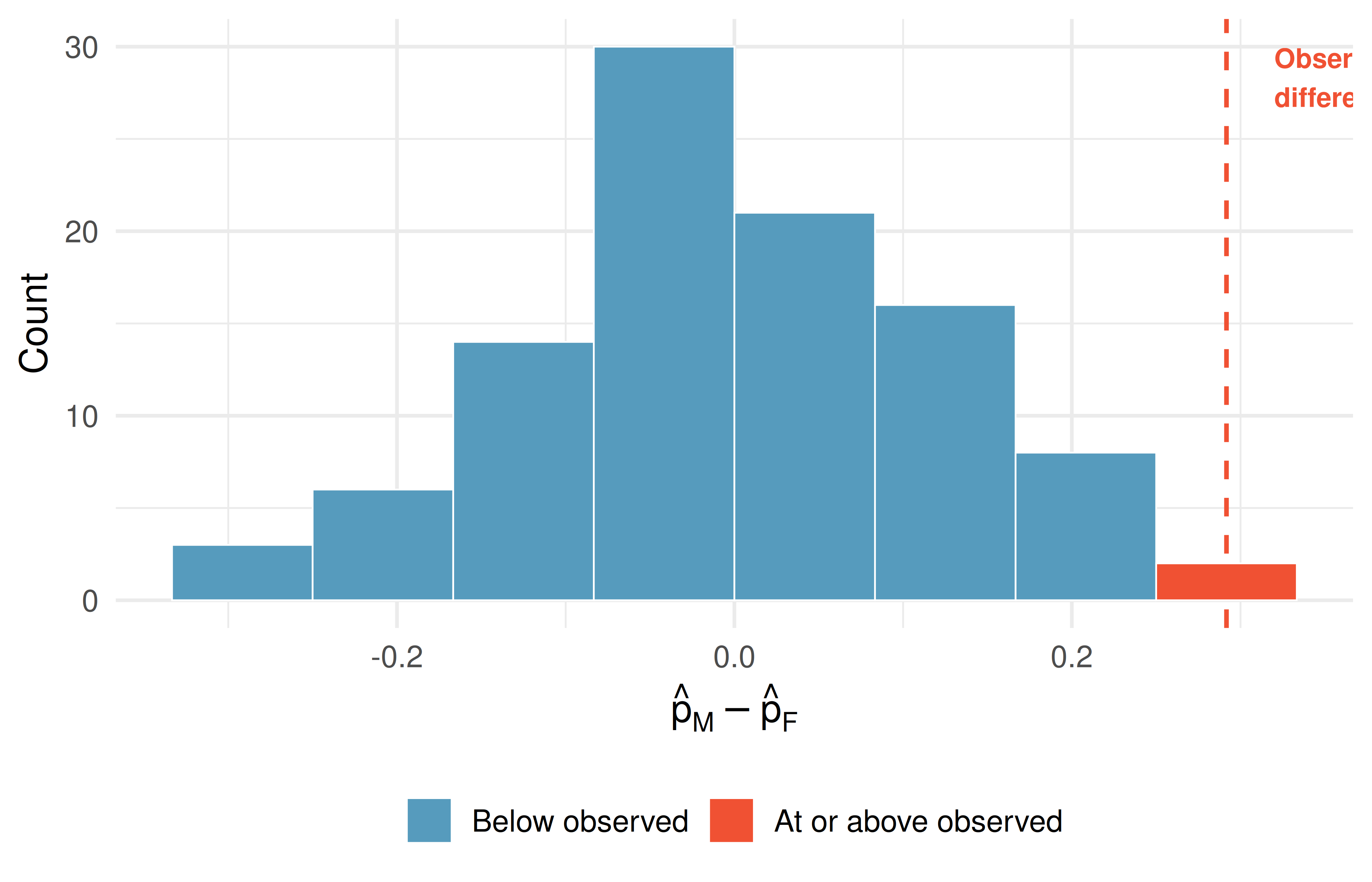
The distribution of these simulated differences is centered around 0. This makes sense: under the null hypothesis, which makes no distinction between male and female files, we would expect the difference to be near zero with some random fluctuation.
How often would you observe a difference of at least 29.2 percentage points according to the randomization distribution? Often, sometimes, rarely, or never?
It appears that a difference of at least 29.2 percentage points under the null hypothesis would only happen about 2% of the time. Such a low probability indicates that observing such a large difference from chance alone is rare.
7.4.4 The conclusion
The difference of 29.2 percentage points is a rare event if there really is no effect of sex on promotion decisions. This provides us with two possible interpretations:
- If \(H_0\) is true: Sex has no effect on promotion decisions, and we observed a difference that is so large it would only happen rarely by chance.
- If \(H_A\) is true: Sex has an effect on promotion decisions, and what we observed was actually due to equally qualified female candidates being discriminated against.
When we conduct formal studies, we reject a null position if the data strongly conflict with it. Since there was only about a 2% probability of obtaining a difference at least as large as 29.2 percentage points under the null hypothesis, we conclude that the data provide strong evidence of sex discrimination. We reject the null hypothesis in favor of the alternative.
Predict → Do → Explain. Open the Randomization Test Walkthrough — a gated activity on the sex-discrimination data. It starts from the observed data and the null hypothesis, then asks you to predict how big one shuffle’s difference should be. You build the null distribution yourself with the +1, +100, and +1000 buttons — each adds a simulated difference to the chart — with a reality-check gate at each stage. It closes with an Explain step where you put in your own words why the shuffle centers at zero, why the tail fraction is the \(p\)-value, and why a different random seed gives a slightly different estimate. Your predictions and explanation save locally in the tool, so you can return to your work on the same device.
Tip
Open sandbox (no scaffolding). Prefer to run the test yourself with your own data? Launch the Randomization Test: Difference in Proportions directly, enter the sex-discrimination table (or your own), generate 1,000 shuffled differences, and read off the tail fraction as the \(p\)-value.
7.5 Case study: opportunity cost
How rational and consistent is the behavior of the typical American college student? Here, we explore whether reminding students that money not spent now can be spent later causes them to be thriftier.
One hundred and fifty students at a university in the southwestern United States were recruited for the study (Frederick et al. 2009). All were given a scenario about purchasing a video on sale for $14.99, and asked to choose between two options. Option (A) — “Buy this entertaining video.” — was the same for everyone. The two groups differed in only one place, option (B):
Control group (B): Not buy this entertaining video.
Treatment group (B): Not buy this entertaining video. Keep the $14.99 for other purchases.
The treatment group’s added clause is a subtle nudge toward opportunity cost — the reminder that money not spent now can be spent later.
The hypotheses are:
- \(H_0\): Reminding students that they can save money for later purchases will not have any impact on their spending decisions.
- \(H_A\): Reminding students that they can save money for later purchases will reduce the chance they will continue with a purchase.
7.5.1 Observed data
The results are summarized below:
| Buy video | Not buy video | Total | |
|---|---|---|---|
| Control | 56 | 19 | 75 |
| Treatment | 41 | 34 | 75 |
| Total | 97 | 53 | 150 |
We define a “success” as a student who chooses not to buy the video. The difference in the proportion choosing not to buy is:
\[\hat{p}_{T} - \hat{p}_{C} = \frac{34}{75} - \frac{19}{75} = 0.453 - 0.253 = 0.200\]
The proportion of students who chose not to buy was 20 percentage points higher in the treatment group. Is this difference of 20 percentage points so large that it is unlikely to have occurred from chance alone?
7.5.2 Simulating under the null
Using the same technique, picture 150 cards — one for each student’s decision. A card’s color records that decision: 53 red cards mean “did not buy” (our “success”) and 97 white cards mean “bought.” Two stacks stand for the treatment and control groups, 75 cards each. Under the null hypothesis the reminder changes no one’s decision, so each card’s color stays fixed — we shuffle all 150 cards and deal them into the two stacks.
If we shuffle and deal the cards into simulated treatment and control stacks, how many red (“did not buy”) cards would we expect in each stack? What would be the expected difference in proportions?
Since the stacks are equal in size, we would expect about \(53/2 \approx 26\) or 27 red cards in each, yielding a difference of roughly 0 percentage points. Due to random chance, we might sometimes observe a little more or fewer than 26–27.
After running 1,000 simulations, the results show that the distribution of simulated differences is centered at 0, as expected under the null hypothesis.
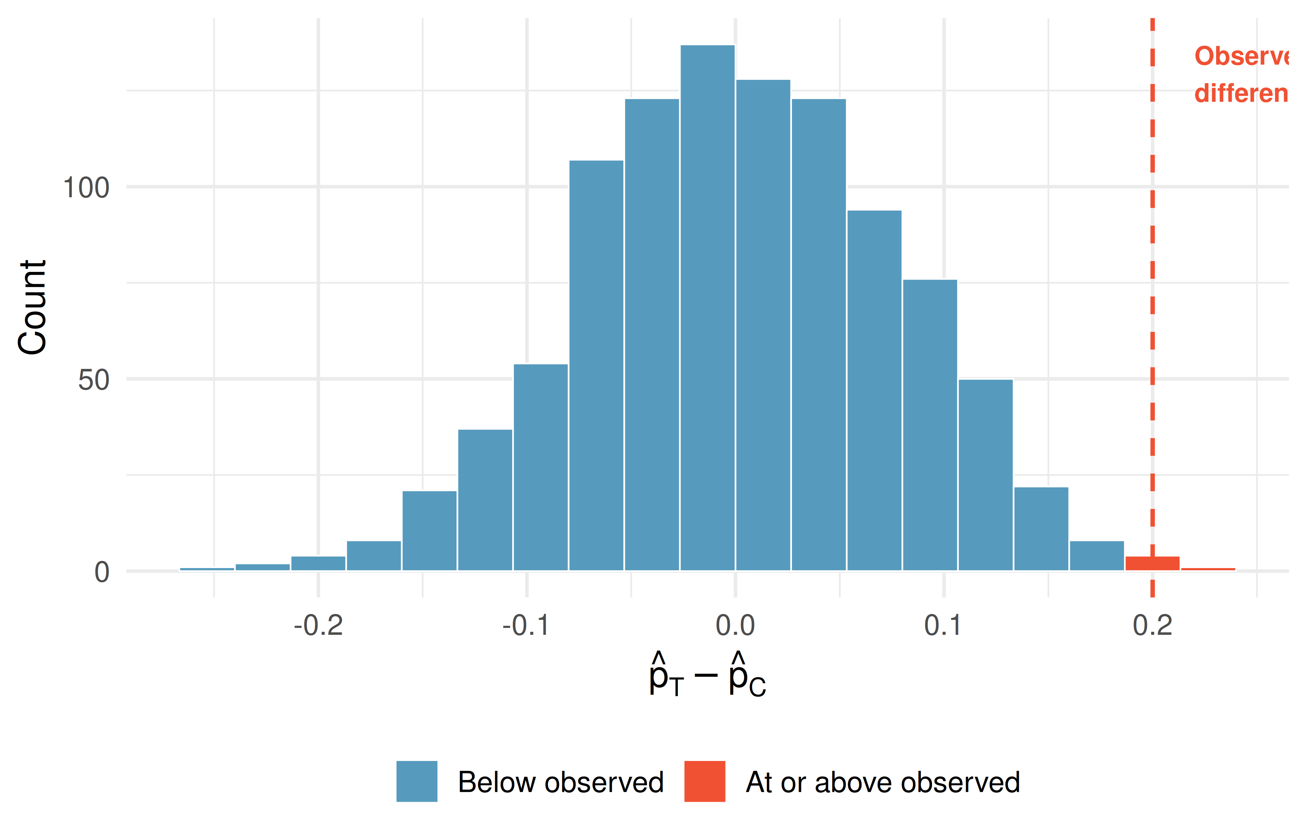
Under the null hypothesis, we would observe a difference of at least +20 percentage points about 0.5% of the time (5 of the 1,000 shuffles). That is very rare! We conclude the data provide strong evidence there is a treatment effect: reminding students that they could spend money later lowers their chance of making a purchase. Because this is an experiment (with random assignment), we can make a causal claim.
7.6 The same idea, for means
Both case studies so far compared two groups on a proportion. But the shuffle never cared what we computed — it breaks the link between the group label and the outcome, whatever that outcome is. Here we run the exact same procedure on a difference in means.
A trainer wonders whether a short warm-up routine improves athletes’ vertical jump. Twenty athletes are randomly assigned to two groups of 10 — one does the warm-up, the other does not — and each athlete’s jump height (in inches) is measured.
The warm-up group averaged 24.05 inches and the control group 22.71 inches, an observed difference of
\[\bar{x}_{\text{warm-up}} - \bar{x}_{\text{control}} = 24.05 - 22.71 = 1.34 \text{ inches.}\]
Could a gap this large come from chance alone, if the warm-up made no real difference?
Under the null hypothesis the warm-up has no effect, so each athlete would have jumped the same height in either group — the label is just a tag. So we do exactly what we did before, changing only the last step:
- Shuffle all 20 jump heights together.
- Deal 10 into a “warm-up” pile and 10 into a “control” pile.
- Compute the difference in mean jump height between the two piles.
The only change from the discrimination study is step 3 — we average the numbers on the cards instead of counting the red ones. Everything else, including why the shuffle is a fair stand-in for chance, is identical.
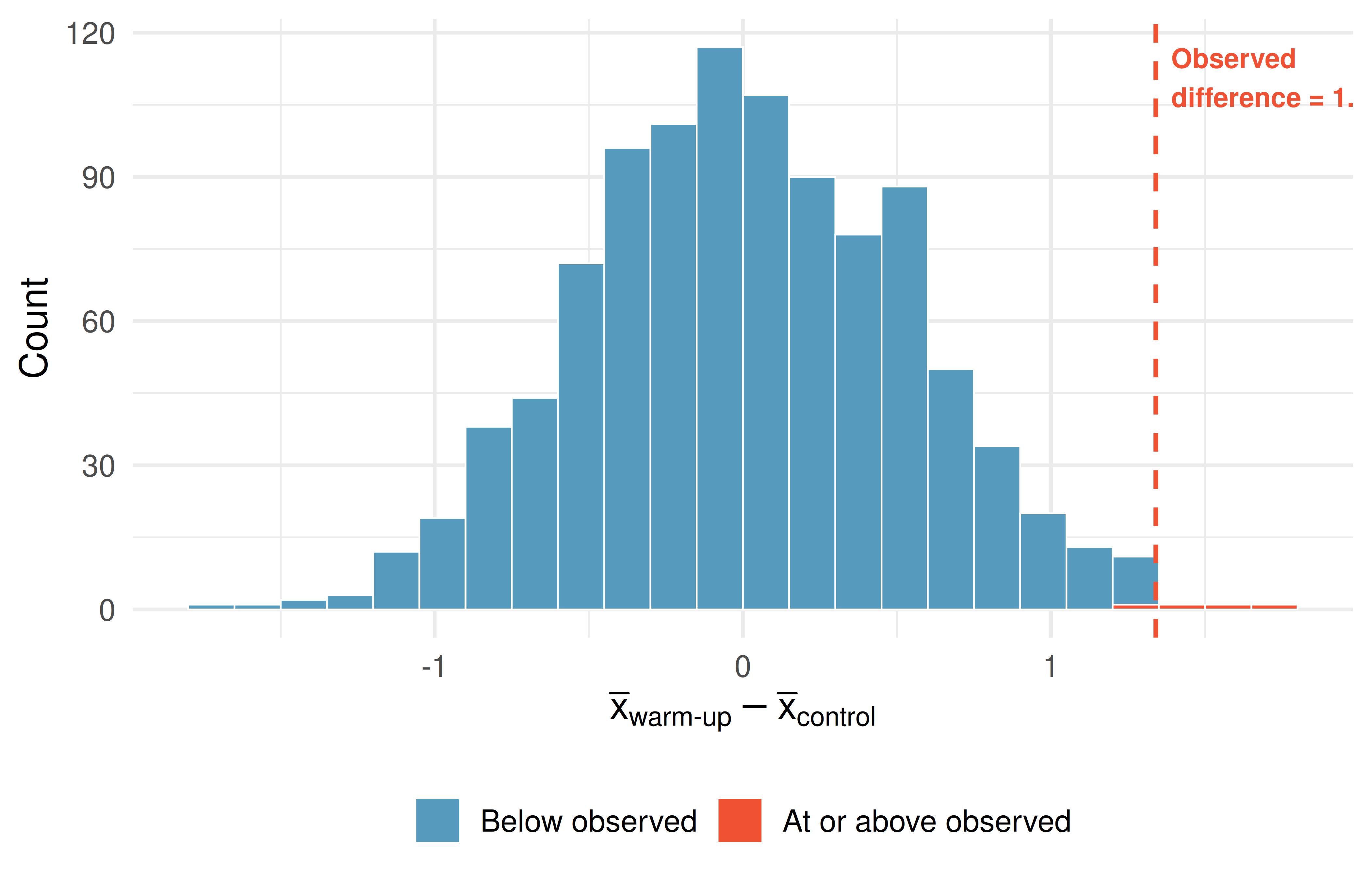
The simulated differences center on zero, exactly as before — under the null, the two groups should differ only by chance. The observed 1.34-inch gap sits far out in the right tail, reached by only a small fraction of shuffles, so the data provide evidence that the warm-up really does improve jump height.
Nothing about the shuffle-and-deal procedure changed between the discrimination study and this one except the statistic we computed at the end. What does that tell you about when a randomization test can be used?
Show answer
The same relabeling logic works for any statistic that compares two groups — a difference in proportions, a difference in means, or something else. As long as the null hypothesis says the group label is unrelated to the outcome, shuffling the labels and recomputing the statistic builds a valid null distribution.7.7 \(p\)-values
The probability we computed in the previous sections — the chance of observing a result as extreme as or more extreme than the one actually observed, if the null hypothesis were true — has a name.
The \(p\)-value is the probability of observing data at least as favorable to the alternative hypothesis as our current dataset, if the null hypothesis were true. We typically use a sample statistic of the data, such as a difference in proportions, to compute the \(p\)-value. (Later, in the theory-based chapters, we standardize a sample statistic into a \(z\)- or \(t\)-score, and that standardized value is what we call the test statistic. In a randomization test we work directly with the sample statistic itself.)
In the sex discrimination study, the sample statistic was the difference in promotion rates. What was the sample statistic in the opportunity cost study?
The sample statistic in the opportunity cost study was the difference in the proportion of students who decided against the video purchase in the treatment and control groups: \(\hat{p}_T - \hat{p}_C = 0.200\).
Interpreting the \(p\)-value.
- A small \(p\)-value (e.g., below 0.05) means that the observed result would be rare if the null hypothesis were true. This is evidence against the null hypothesis.
- A large \(p\)-value (e.g., above 0.10) means that the observed result is not particularly unusual under the null hypothesis. The data do not provide strong evidence against the null hypothesis.
- The \(p\)-value is not the probability that the null hypothesis is true. It is the probability of the observed data (or more extreme data) given that the null hypothesis is true.
A common mistake is to interpret the \(p\)-value as the probability that the null hypothesis is true (e.g., “there is a 2% chance that sex has no effect on promotions”). This is incorrect. The \(p\)-value tells us how surprising the data would be if the null hypothesis were true, not how likely the null hypothesis is to be true.
7.8 Statistical discernibility
We say that the data provide statistically discernible evidence against the null hypothesis if the \(p\)-value is less than a predetermined threshold called the discernibility level, denoted \(\alpha\) (the Greek letter alpha).
A note on the vocabulary
Traditionally this result has been called statistically significant, and the threshold \(\alpha\) the significance level — terms you will still see in most other books. Because significant in everyday English suggests large or important, which a small but genuinely detectable effect may not be, we follow Introduction to Modern Statistics and instead call the result statistically discernible and the threshold the discernibility level.
The most commonly used discernibility level is \(\alpha = 0.05\), meaning we reject the null hypothesis when the \(p\)-value is less than 5%. However, there is nothing magical about 0.05 — it is a convention, and in some fields or applications a stricter (e.g., 0.01) or more lenient (e.g., 0.10) threshold may be appropriate.
In the opportunity cost study, we found that a difference of at least 20 percentage points would occur only about 5-in-1,000 times if the reminder had no influence on student decisions. The \(p\)-value is approximately 0.005. Would you classify this as statistically discernible?
Yes. Since \(p\text{-value} \approx 0.005 < 0.05 = \alpha\), the data provide statistically discernible evidence that US college students were actually influenced by the reminder.
What “statistically discernible” does and does not mean.
“Statistically discernible” means the \(p\)-value fell below the chosen discernibility level. It does not necessarily mean the effect is large or practically important. A very large sample can detect a tiny difference as “statistically discernible” even if the difference is too small to matter in practice.
Conversely, “not statistically discernible” does not mean there is no effect. It may simply mean the sample was too small to detect the effect.
7.8.1 Decision framework
The logic of hypothesis testing follows a consistent pattern:
| If the \(p\)-value is… | Then we… | Because… |
|---|---|---|
| Less than \(\alpha\) | Reject \(H_0\) | The data are unlikely under \(H_0\); evidence supports \(H_A\) |
| Greater than or equal to \(\alpha\) | Fail to reject \(H_0\) | The data are not sufficiently unusual under \(H_0\) |
A researcher tests whether a new teaching method improves exam scores compared to the standard method. The \(p\)-value from the randomization test is 0.12. Using \(\alpha = 0.05\), what conclusion should the researcher draw?
Show answer
Since \(p\text{-value} = 0.12 > 0.05 = \alpha\), the researcher fails to reject the null hypothesis. The data do not provide sufficient evidence that the new teaching method improves exam scores. This does not mean the new method is ineffective — only that this study did not produce enough evidence to conclude it is effective.7.9 Two-sided tests
In the sex discrimination study, we looked for differences in one direction only — whether female candidates were promoted at a lower rate. This is called a one-sided (or one-tailed) test. The alternative hypothesis specified a direction:
\[H_A: p_M - p_F > 0 \quad \text{(males promoted at a higher rate)}\]
Sometimes, however, we are interested in detecting a difference in either direction. For example, if we are studying whether a new drug changes the recovery rate compared to the standard treatment (it could raise it or lower it), we would use a two-sided (or two-tailed) test:
\[H_A: p_1 \neq p_2 \quad \text{(the proportions are different, in either direction)}\]
In a one-sided test, the alternative hypothesis specifies a direction (greater than or less than). The \(p\)-value is computed as the proportion of the randomization distribution in one tail.
In a two-sided test, the alternative hypothesis does not specify a direction (just “different”). The \(p\)-value is computed as the proportion of the randomization distribution in both tails — values at least as extreme as the observed statistic in either direction.
Suppose we are testing whether a coin is fair. We flip it 100 times and get 60 heads.
- One-sided (\(H_A: p > 0.5\)): The \(p\)-value counts only simulations with 60 or more heads.
- Two-sided (\(H_A: p \neq 0.5\)): The \(p\)-value counts simulations with 60 or more heads and simulations with 40 or fewer heads (equally extreme in the other direction).
For a symmetric randomization distribution, the two-sided \(p\)-value is approximately twice the one-sided \(p\)-value. If the one-sided \(p\)-value is 0.03, the two-sided \(p\)-value is approximately 0.06.
A researcher wants to know if a new fertilizer changes plant growth compared to no fertilizer. Should this be a one-sided or two-sided test? Write the hypotheses using appropriate notation, where \(\mu_T\) is the mean growth with fertilizer and \(\mu_C\) is the mean growth without.
Show answer
This should be a two-sided test because the fertilizer could either increase or decrease growth (perhaps it has a toxic effect in some soils). The hypotheses are: \(H_0: \mu_T - \mu_C = 0\) (no difference in mean growth) and \(H_A: \mu_T - \mu_C \neq 0\) (the fertilizer changes mean growth, in either direction).Choosing one-sided vs. two-sided.
- Use a one-sided test when you have a specific directional hypothesis before looking at the data. For example, “we believe this drug lowers blood pressure.”
- Use a two-sided test when you want to detect a difference in either direction, or when you are not sure which direction the difference might go.
- When in doubt, use a two-sided test. It is the more conservative choice and is less susceptible to bias from choosing the direction after seeing the data.
7.10 The randomization test procedure: a summary
We can summarize the randomization test procedure as follows:
Frame the research question in terms of hypotheses. The null hypothesis (\(H_0\)) usually represents no difference or no effect. The alternative hypothesis (\(H_A\)) represents the claim of interest.
Collect data. If the research question focuses on associations but not causation, use an observational study. If you want to establish a causal connection, use an experiment with random assignment.
Model what would happen under the null hypothesis. Shuffle (randomize) the data to break any association between the explanatory and response variables. Compute the sample statistic for each shuffle. Repeat many times to build the randomization distribution (also called the null distribution).
Compute the \(p\)-value. Determine what proportion of the randomization distribution is at least as extreme as the observed sample statistic.
Draw a conclusion. If the \(p\)-value is small (less than \(\alpha\)), reject \(H_0\) and conclude there is evidence for \(H_A\). If the \(p\)-value is not small, fail to reject \(H_0\). Write the conclusion in context, in plain language.
See it in action. Open the Randomization Test: Difference in Proportions to run the full procedure on your own data — and watch how the \(p\)-value shifts when you change the sample size or the magnitude of the observed difference.
Testing a single proportion by simulation
This chapter focused on comparing two groups because that is the most common use of a randomization test. The same simulate-under-\(H_0\) logic also works for a single sample against a claimed proportion — instead of shuffling group labels, you draw new samples from a modeled null population. That one-sample simulation test is developed in the inference for proportions chapter (see the “Building the null distribution by simulation” section).
7.11 Chapter review
7.11.1 Summary
- A hypothesis test evaluates two competing claims: the null hypothesis (\(H_0\)), which represents no effect or no difference, and the alternative hypothesis (\(H_A\)), which represents the claim under investigation.
- A randomization test (or permutation test) assesses the null hypothesis by shuffling the data to simulate what would happen if there were truly no effect. The collection of simulated sample statistics forms the randomization distribution.
- The sample statistic is the summary value computed from the data (e.g., a difference in proportions) that we use to evaluate the hypotheses.
- The \(p\)-value is the probability of observing a sample statistic at least as extreme as the one observed, assuming the null hypothesis is true. It quantifies the strength of the evidence against \(H_0\).
- We reject \(H_0\) when the \(p\)-value is less than the discernibility level \(\alpha\) (commonly 0.05). This is called a statistically discernible result.
- A one-sided test looks for effects in a specified direction; a two-sided test looks for effects in either direction.
- Failing to reject \(H_0\) is not the same as proving \(H_0\) is true.
- Statistical discernibility does not imply practical importance.
7.11.2 Key terms
| Term | Definition |
|---|---|
| Hypothesis test | A formal procedure for evaluating competing claims using data |
| Null hypothesis (\(H_0\)) | The claim of no effect or no difference; the skeptical position |
| Alternative hypothesis (\(H_A\)) | The claim that there is an effect or difference |
| Randomization test | A hypothesis test that builds a null distribution by shuffling data |
| Randomization distribution | The distribution of the sample statistic under repeated randomizations |
| Sample statistic | The summary value computed from the data (e.g., a difference in proportions) used to evaluate the hypotheses |
| \(p\)-value | Probability of observing a result as extreme as or more extreme than the data, if \(H_0\) is true |
| Discernibility level (\(\alpha\)) | The threshold below which the \(p\)-value leads us to reject \(H_0\) |
| Statistically discernible | A result whose \(p\)-value falls below \(\alpha\) |
| One-sided test | Alternative hypothesis specifies a direction |
| Two-sided test | Alternative hypothesis does not specify a direction |
7.12 Exercises
Answers to odd-numbered exercises are provided in the Exercise Solutions appendix at the back of the book.
- Hypotheses. For each of the research statements below, note whether it represents a null hypothesis claim or an alternative hypothesis claim.
The number of hours that grade-school children spend doing homework predicts their future success on standardized tests.
King cheetahs on average run the same speed as standard spotted cheetahs.
For a particular student, the probability of correctly answering a 5-option multiple choice test is larger than 0.2 (i.e., better than guessing).
The mean length of African elephant tusks has changed over the last 100 years.
The risk of facial clefts is equal for babies born to mothers who take folic acid supplements compared with those from mothers who do not.
Caffeine intake during pregnancy affects mean birth weight.
The probability of getting in a car accident is the same if using a cell phone than if not using a cell phone.
- True null hypothesis. Unbeknownst to you, let’s say that the null hypothesis is actually true in the population. You plan to run a study anyway.
If the level of discernibility you choose (i.e., the cutoff for your p-value) is 0.05, how likely is it that you will mistakenly reject the null hypothesis?
If the level of discernibility you choose (i.e., the cutoff for your p-value) is 0.01, how likely is it that you will mistakenly reject the null hypothesis?
If the level of discernibility you choose (i.e., the cutoff for your p-value) is 0.10, how likely is it that you will mistakenly reject the null hypothesis?
- Identify hypotheses, I. Write the null and alternative hypotheses in words and then symbols for each of the following situations.
New York is known as “the city that never sleeps”. A random sample of 25 New Yorkers were asked how much sleep they get per night. Do these data provide convincing evidence that New Yorkers on average sleep less than 8 hours a night?
Employers at a firm are worried about the effect of March Madness, a basketball championship held each spring in the US, on employee productivity. They estimate that on a regular business day employees spend on average 15 minutes of company time checking personal email, making personal phone calls, etc. They also collect data on how much company time employees spend on such non- business activities during March Madness. They want to determine if these data provide convincing evidence that employee productivity decreases during March Madness.
- Identify hypotheses, II. Write the null and alternative hypotheses in words and using symbols for each of the following situations.
Since 2008, chain restaurants in California have been required to display calorie counts of each menu item. Prior to menus displaying calorie counts, the average calorie intake of diners at a restaurant was 1100 calories. After calorie counts started to be displayed on menus, a nutritionist collected data on the number of calories consumed at this restaurant from a random sample of diners. Do these data provide convincing evidence of a difference in the average calorie intake of a diners at this restaurant?
Based on the performance of those who took the GRE exam between July 1, 2004 and June 30, 2007, the average Verbal Reasoning score was calculated to be 462. In 2021 the average verbal score was slightly higher. Do these data provide convincing evidence that the average GRE Verbal Reasoning score has changed since 2021?
- Side effects of Avandia. Rosiglitazone is the active ingredient in the controversial type 2 diabetes medicine Avandia and has been linked to an increased risk of serious cardiovascular problems such as stroke, heart failure, and death. A common alternative treatment is Pioglitazone, the active ingredient in a diabetes medicine called Actos. In a nationwide retrospective observational study of 227,571 Medicare beneficiaries aged 65 years or older, it was found that 2,593 of the 67,593 patients using Rosiglitazone and 5,386 of the 159,978 using Pioglitazone had serious cardiovascular problems. These data are summarized in the contingency table below. (Graham et al. 2010)
| Treatment | No | Yes | Total |
|---|---|---|---|
| Pioglitazone | 154,592 | 5,386 | 159,978 |
| Rosiglitazone | 65,000 | 2,593 | 67,593 |
| Total | 219,592 | 7,979 | 227,571 |
Determine if each of the following statements is true or false. If false, explain why. Be careful: The reasoning may be wrong even if the statement’s conclusion is correct. In such cases, the statement should be considered false.
Since more patients on Pioglitazone had cardiovascular problems (5,386 vs. 2,593), we can conclude that the rate of cardiovascular problems for those on a Pioglitazone treatment is higher.
The data suggest that diabetic patients who are taking Rosiglitazone are more likely to have cardiovascular problems since the rate of incidence was (2,593 / 67,593 = 0.038) 3.8% for patients on this treatment, while it was only (5,386 / 159,978 = 0.034) 3.4% for patients on Pioglitazone.
The fact that the rate of incidence is higher for the Rosiglitazone group proves that Rosiglitazone causes serious cardiovascular problems.
Based on the information provided so far, we cannot tell if the difference between the rates of incidences is due to a relationship between the two variables or due to chance.
What proportion of all patients had cardiovascular problems?
If the type of treatment and having cardiovascular problems were independent, how many patients in the Rosiglitazone group would we expect to have had cardiovascular problems?
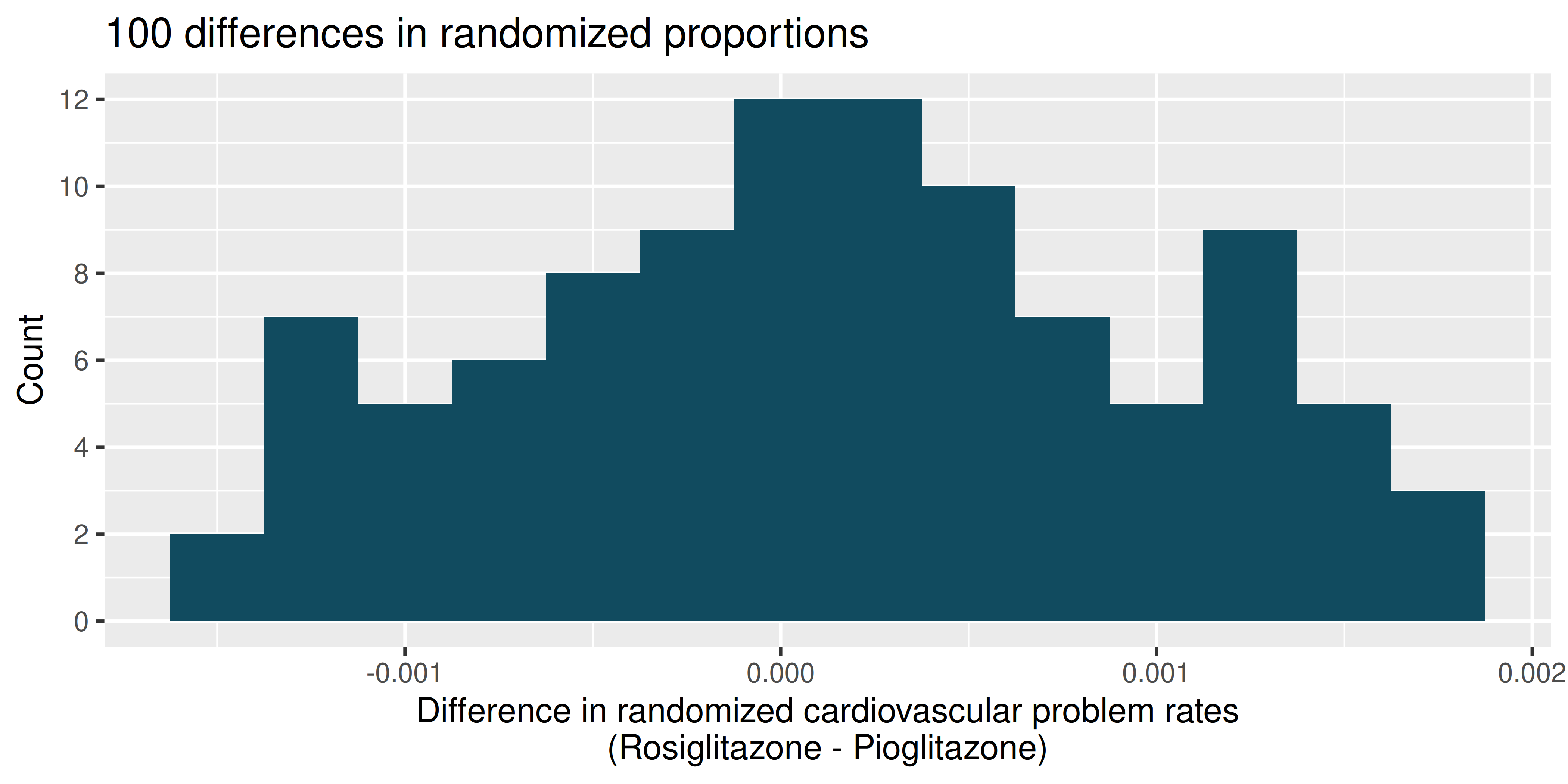
We can investigate the relationship between outcome and treatment in this study using a randomization technique. While in reality we would carry out the simulations required for randomization using statistical software, suppose we actually simulate using index cards. In order to simulate from the independence model, which states that the outcomes were independent of the treatment, we write whether each patient had a cardiovascular problem on cards, shuffled all the cards together, then deal them into two groups of size 67,593 and 159,978. We repeat this simulation 100 times and each time record the difference between the proportions of cards that say “Yes” in the Rosiglitazone and Pioglitazone groups. Use the histogram of these differences in proportions to answer the following questions.
What are the claims being tested?
Compared to the number calculated in part (b), which would provide more support for the alternative hypothesis, higher or lower proportion of patients with cardiovascular problems in the Rosiglitazone group?
What do the simulation results suggest about the relationship between taking Rosiglitazone and having cardiovascular problems in diabetic patients?
- Heart transplants. The Stanford University Heart Transplant Study was conducted to determine whether an experimental heart transplant program increased lifespan. Each patient entering the program was designated an official heart transplant candidate, meaning that they were gravely ill and would most likely benefit from a new heart. Some patients got a transplant and some did not. The variable
transplantindicates which group the patients were in; patients in the treatment group got a transplant and those in the control group did not. Of the 34 patients in the control group, 30 died. Of the 69 people in the treatment group, 45 died. Another variable calledsurvivedwas used to indicate whether the patient was alive at the end of the study. (Turnbull, Brown, and Hu 1974)
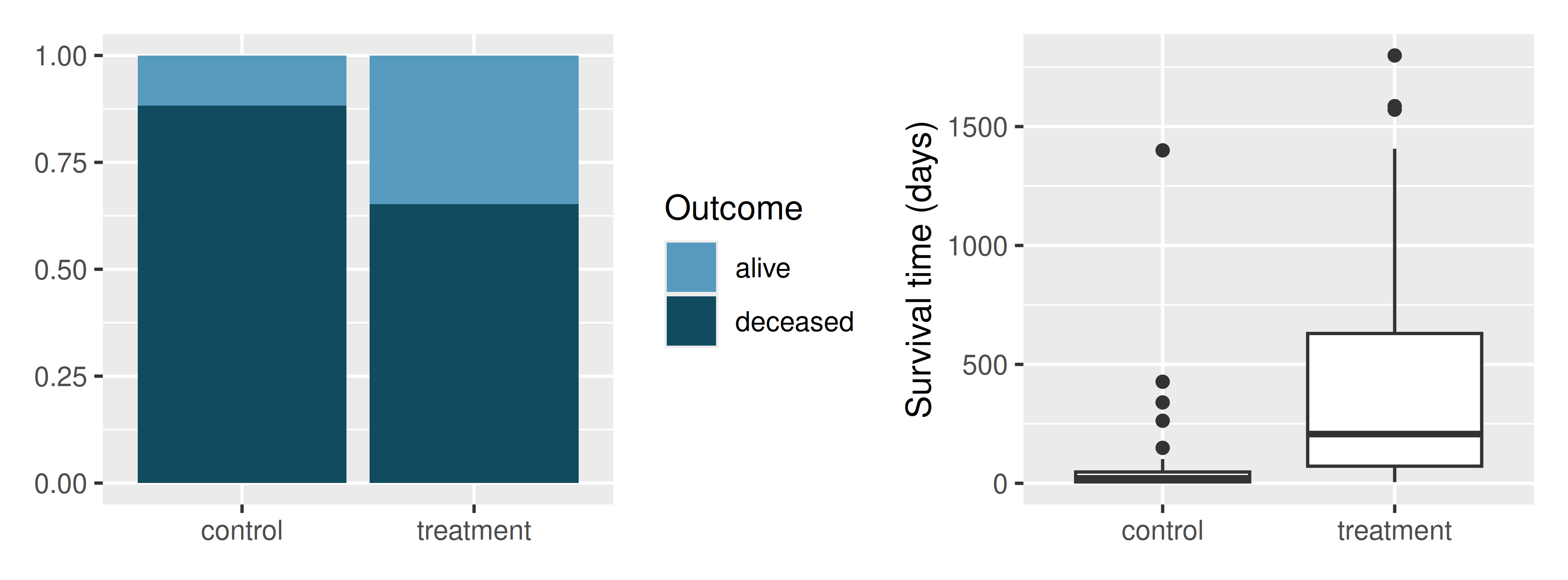
Does the stacked bar plot indicate that survival is independent of whether the patient got a transplant? Explain your reasoning.
What do the box plots suggest about the efficacy of heart transplants.
What proportions of patients in the treatment and control groups died?
One approach for investigating whether the treatment is discernably effective is randomization testing.
What are the claims being tested?
The paragraph below describes the set up for a randomization test, if we were to do it without using statistical software. Fill in the blanks with a number or phrase.
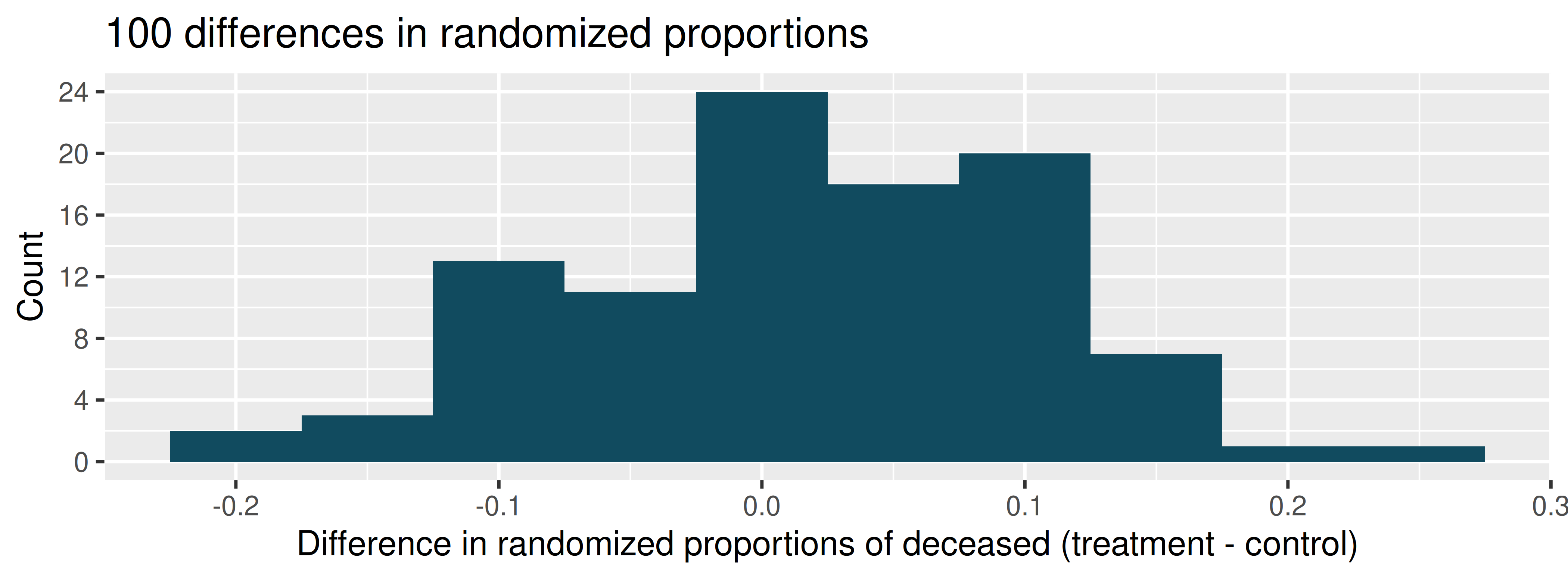
We write alive on \(\rule{1.25cm}{0.5pt}\) cards representing patients who were alive at the end of the study, and deceased on \(\rule{1.25cm}{0.5pt}\) cards representing patients who were not. Then, we shuffle these cards and split them into two groups: one group of size \(\rule{1.25cm}{0.5pt}\) representing treatment, and another group of size \(\rule{1.25cm}{0.5pt}\) representing control. We calculate the difference between the proportion of cards in the treatment and control groups (treatment - control) and record this value. We repeat this 100 times to build a distribution centered at \(\rule{1.25cm}{0.5pt}\). Lastly, we calculate the proportion of simulations where the simulated differences in proportions are \(\rule{1.25cm}{0.5pt}\). If this proportion is low, we conclude that it is unlikely to have observed such an outcome by chance and that the null hypothesis should be rejected in favor of the alternative.
- What do the simulation results shown below suggest about the effectiveness of heart transplants?
StatLens Exercises
These exercises focus on the parts of a randomization test a calculator can’t do for you: framing the question, picking the right shuffling scheme, reading the null distribution, and interpreting a p-value without falling into the standard traps. Let StatLens do the arithmetic.
Frame the question. A trial randomly assigns 90 students to either an online tutoring program or a control group, then measures their final exam scores. The mean score in the tutoring group is 4.2 points higher than in the control group.
- What is the parameter of interest? Describe it in words.
- Write \(H_0\) and \(H_A\) for testing whether tutoring improves exam scores. Is the test one-sided or two-sided, and why?
- The randomization test will simulate the “no effect” world by shuffling group labels across students. Why is shuffling labels the right way to simulate \(H_0\) here, and what feature of the study design makes shuffling labels valid?
Choose the procedure. For each scenario, name the randomization shuffle you would use — shuffle group labels (independent groups), shuffle paired-difference signs (paired data), shuffle the values of one variable (correlation/independence), or a Bernoulli null simulation (one proportion vs. a fixed value).
- Did a coin biased toward heads come up “heads” more than 50% of the time in 100 tosses?
- Are male and female job applicants offered different mean starting salaries?
- Do students score higher on a test taken after a study skills workshop compared to before?
- Is hours of TV per week associated with hours of sleep per night?
- Do four different fertilizer brands produce different mean yields?
Read the null distribution. Open the Randomization Test — Difference in Proportions (the gated sex-discrimination walkthrough). Step through it until you have the full null distribution (the walkthrough’s +100 and +1000 steps, about 1,100 shuffled differences) in front of you.
- Where is the null distribution centered? Why does it have to be centered there, by construction?
- The observed sample difference is marked on the dotplot. Roughly what proportion of the shuffled differences are at least as extreme as the observed one (one-sided)? That proportion is the p-value.
- Suppose the observed difference had landed near the middle of the null distribution instead. What would the p-value be approximately, and what would you conclude?
Run it and interpret it (means). Open the Randomization Test for Difference in Means with any two-group numeric dataset.
Run 1000 shuffles and read off the p-value. State your decision at \(\alpha = 0.05\).
Write a one-sentence conclusion in context.
Re-run the test with only 100 shuffles, then with 10000 shuffles. How does the p-value change? Why do we usually report a number that comes from “more shuffles, not fewer”?
Which statement is the correct interpretation of a p-value of 0.03?
- There is a 3% probability that the null hypothesis is true.
- If the two groups really had the same mean, we would see a difference at least as extreme as ours in about 3% of randomly assigned studies.
- The probability that the alternative hypothesis is true is 0.97.
Simulation as a sanity check on the normal approximation. A textbook says: “When the sample sizes are large and the data are not too skewed, the randomization distribution of \(\bar{x}_1 - \bar{x}_2\) is approximately normal.” You will check this by eye.
- Open any moderate-\(n\) two-group numeric dataset in the randomization test tool and run 5000 shuffles. Describe the shape, center, and spread of the resulting null distribution.
- Why does the spread of the null distribution tell you the standard error of \(\bar{x}_1 - \bar{x}_2\) — and why does that mean a randomization test essentially “discovers” the same SE the \(t\)-formula computes from \(s_1\), \(s_2\), \(n_1\), \(n_2\)?
- Now try the same on a small, skewed dataset (say \(n_1 = n_2 = 6\), with one outlier). Is the null distribution still approximately normal? If you ran a two-sample \(t\)-test on this same data, would the \(t\) distribution be a good match for the randomization distribution? Where would they disagree?
- A student claims that the randomization test “only works for large samples.” Why is this exactly backwards — which test works better in small samples, the \(t\)-test or the randomization test, and why?
Frederick, S., N. Novemsky, J. Wang, R. Dhar, and S. Nowlis. 2009. “Opportunity Cost Neglect.” Journal of Consumer Research 36 (4): 553–61.
Graham, D. J., R. Ouellet-Hellstrom, T. E. MaCurdy, F. Ali, C. Sholley, C. Worrall, and J. A. Kelman. 2010. “Risk of Acute Myocardial Infarction, Stroke, Heart Failure, and Death in Elderly Medicare Patients Treated with Rosiglitazone or Pioglitazone.” JAMA 304 (4): 411. https://doi.org/10.1001/jama.2010.920.
Rosen, B., and T. H. Jerdee. 1974. “Influence of Sex Role Stereotypes on Personnel Decisions.” Journal of Applied Psychology 59 (1): 9. https://doi.org/doi.org/10.1037/h0035834.
Turnbull, B., B. Brown, and M. Hu. 1974. “Survivorship of Heart Transplant Data.” Journal of the American Statistical Association 69: 74–80. https://doi.org/10.1080/01621459.1974.10480130.