Project — Analysis of Variance. Carry out the analysis in Jamovi (or R) and communicate the result. ANOVA asks whether any of several group means differ; the graded skills are framing that question, checking conditions, and interpreting the F-test in context.
The question
In baseball, a player’s on-base percentage (OBP) measures how often they reach base. Do players at different field positions tend to get on base at different rates?
Do mean OBP values differ across infielders, outfielders, and catchers?
The data
mlb_players_18 holds 2018 Major League Baseball players. You’ll use OBP and position. We restrict to position players with regular playing time (at least 100 at-bats) and group positions into Infield, Outfield, and Catcher (pitchers and designated hitters are set aside). The R tab builds that grouping; in Jamovi you would create the same grouped column.
Plan it first
Variables. Identify the numerical response and the categorical explanatory variable, and how many groups it has.
Hypotheses. State \(H_0\) (all group means equal) and \(H_A\) (at least one differs). Why is \(H_A\)not “all means are different”?
Procedure. One numerical outcome across three groups → one-way ANOVA (the F-test), not a pile of \(t\)-tests. Why not just run all the pairwise \(t\)-tests?
After ANOVA. If F is discernible, what additional step tells you which positions differ?
# Observed F statistic, then a randomization (permutation) F distributionobs_F <- d |>specify(OBP ~ pos_group) |>calculate(stat ="F")obs_F
Response: OBP (numeric)
Explanatory: pos_group (factor)
# A tibble: 1 × 1
   stat
  <dbl>
1  5.08
set.seed(145)null_F <- d |>specify(OBP ~ pos_group) |>hypothesize(null ="independence") |>generate(reps =1000, type ="permute") |>calculate(stat ="F")null_F |>get_p_value(obs_stat = obs_F, direction ="greater")
# A tibble: 1 × 1
  p_value
    <dbl>
1   0.006
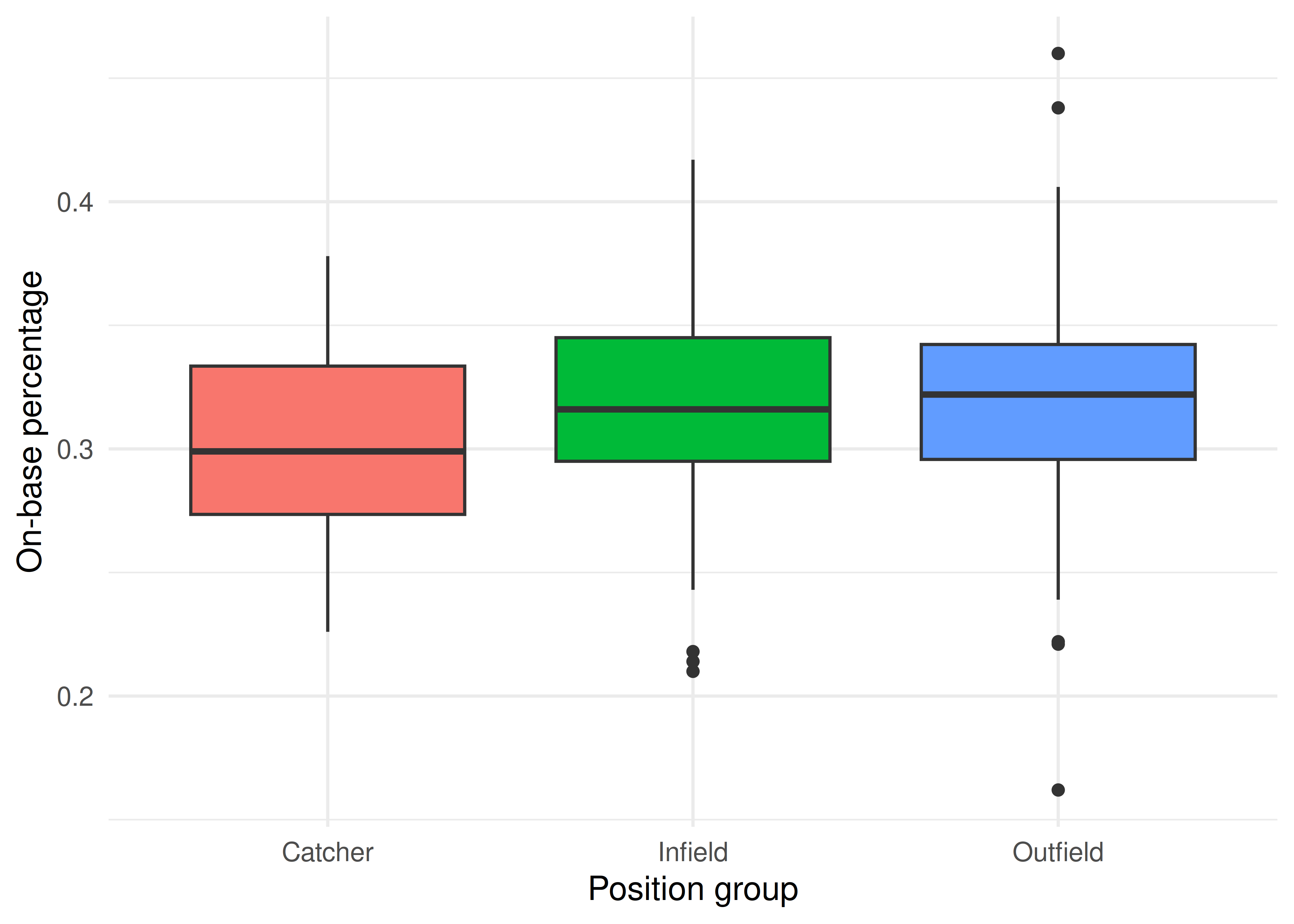
ggplot(d, aes(pos_group, OBP, fill = pos_group)) +geom_boxplot(show.legend =FALSE) +labs(x ="Position group", y ="On-base percentage") +theme_minimal(base_size =13)
On-base percentage by position group for regular MLB position players in 2018.
Your deliverable
Submit a short report containing all of:
Graphic — labeled boxplots of OBP by position group.
Numerical result — the group means, the F-statistic, and the p-value.
Conditions — one sentence on the ANOVA conditions (independent groups, roughly normal, similar spreads).
Conclusion in context — 3–4 sentences: is there discernible evidence that mean OBP differs by position group? If so, note that ANOVA alone doesn’t say which groups differ, and report what the post-hoc comparison found (if you ran it).
One limitation — e.g., position grouping is a simplification; 2018 only.
How it’s graded
Criterion
What we look for
Appropriate, labeled graphic
boxplots by group, axes labeled
Procedure & conditions
one-way ANOVA identified; conditions addressed
Correct numerical result
group means, F, p-value reported correctly
Conclusion in context
discernibility + “F doesn’t say which pair” + post-hoc if used
Communication
clear, correct interpretation
Warm up first. Build intuition for between- vs. within-group variation in the ANOVA tool before writing your report.