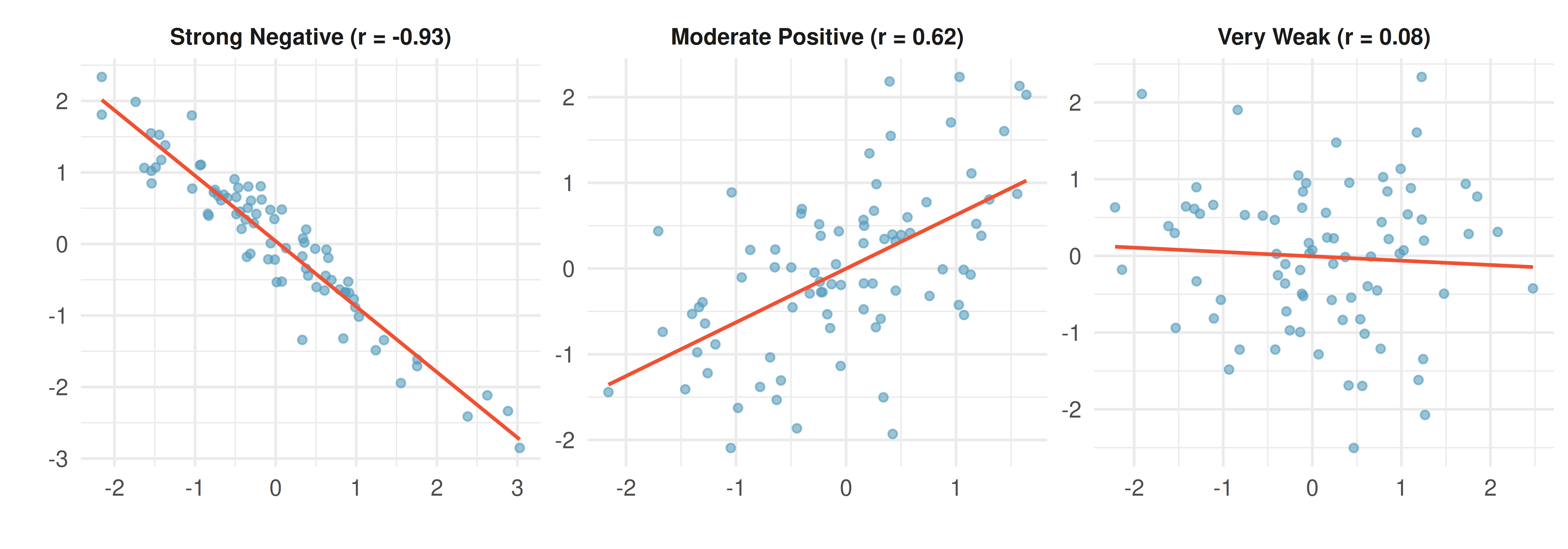
20 Linear Regression
Linear regression is a powerful statistical technique for describing the relationship between two quantitative variables. Many people have some familiarity with regression just from reading the news, where straight lines are overlaid on scatterplots. In this chapter, we build on the ideas of correlation from the previous chapter to develop the least squares regression line. We learn how to interpret the slope and intercept, use residuals to assess model fit, quantify the strength of the model with \(R^2\), and perform inference on the slope to test whether a linear relationship exists in the population.
20.1 Fitting a line to data
Linear regression is the statistical method for fitting a line to data where the relationship between two variables, \(x\) and \(y\), can be modeled by a straight line with some error:
\[y = b_0 + b_1 x + e\]
The values \(b_0\) and \(b_1\) represent the model’s intercept and slope, respectively, and the error is represented by \(e\). These values are calculated from the data – they are sample statistics. If the observed data are a random sample from a target population, these values are point estimates for the population parameters \(\beta_0\) and \(\beta_1\).
When we use \(x\) to predict \(y\), we call \(x\) the predictor variable (or explanatory variable) and \(y\) the outcome variable (or response variable). We often write the model without the error term when focusing on the predicted average outcome:
\[\hat{y} = b_0 + b_1 x\]
The “hat” on \(y\) signifies that this is a predicted (estimated) value.
It is rare for all data to fall perfectly on a straight line. Instead, data more commonly appear as a cloud of points, where the trend may be strong or weak.
There are also cases where fitting a straight line is inappropriate, even if there is a clear relationship between the variables. When the relationship is nonlinear, a linear model can be misleading.
20.1.1 Using linear regression to predict possum head lengths
Researchers captured 104 brushtail possums in Australia and took body measurements. We consider total body length (cm) as the predictor to predict head length (mm).
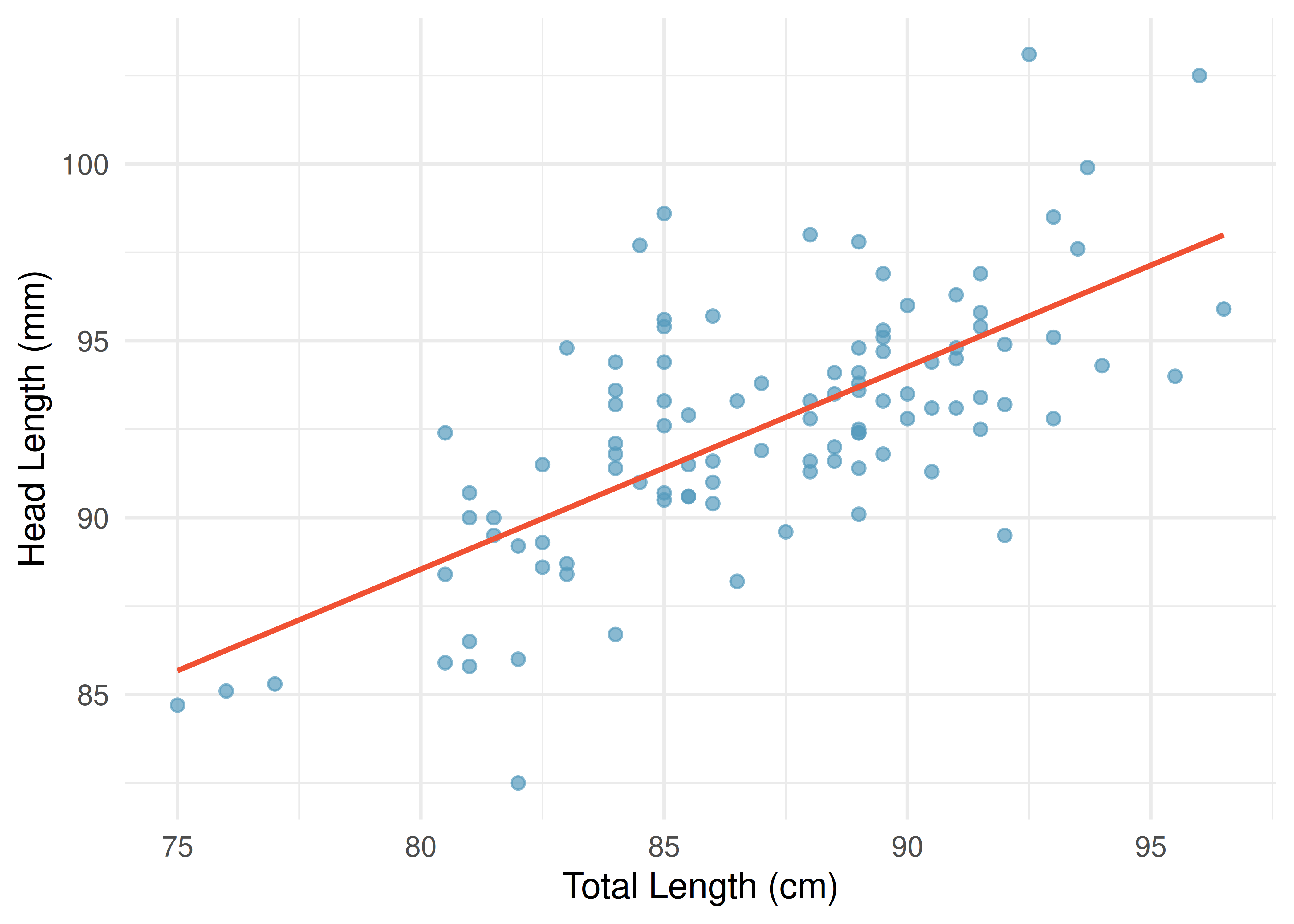
The equation for this line is:
\[\hat{y} = 41 + 0.59x\]
We can use this line to make predictions. For instance, the equation predicts a possum with a total length of 80 cm will have a head length of:
\[\hat{y} = 41 + 0.59 \times 80 = 88.2 \text{ mm}\]
This estimate may be viewed as an average: the equation predicts that possums with a total length of 80 cm will have an average head length of 88.2 mm.
20.2 Residuals
Residuals are the leftover variation in the data after accounting for the model fit:
\[\text{Data} = \text{Fit} + \text{Residual}\]
Each observation has a residual. If an observation is above the regression line, its residual is positive. If it is below the line, the residual is negative.
Residual: Difference between observed and expected.
The residual of the \(i^{th}\) observation \((x_i, y_i)\) is the difference between the observed outcome and the predicted outcome:
\[e_i = y_i - \hat{y}_i\]
We identify \(\hat{y}_i\) by plugging \(x_i\) into the model.
The linear fit is \(\hat{y} = 41 + 0.59x\). Compute the residual for the observation \((76.0, 85.1)\).
First compute the predicted value: \(\hat{y} = 41 + 0.59 \times 76.0 = 85.84\). The residual is \(e = 85.1 - 85.84 = -0.74\) mm. The negative residual indicates that the model overpredicted head length for this possum.
If a model underestimates an observation, will the residual be positive or negative? What about if it overestimates?
Show answer
If a model underestimates an observation, the residual is positive (the actual value exceeds the prediction). If it overestimates, the residual is negative.20.2.1 Residual plots
Residuals are helpful in evaluating how well a linear model fits a dataset. We display them in a residual plot, where the horizontal axis shows the predicted values and the vertical axis shows the residuals.
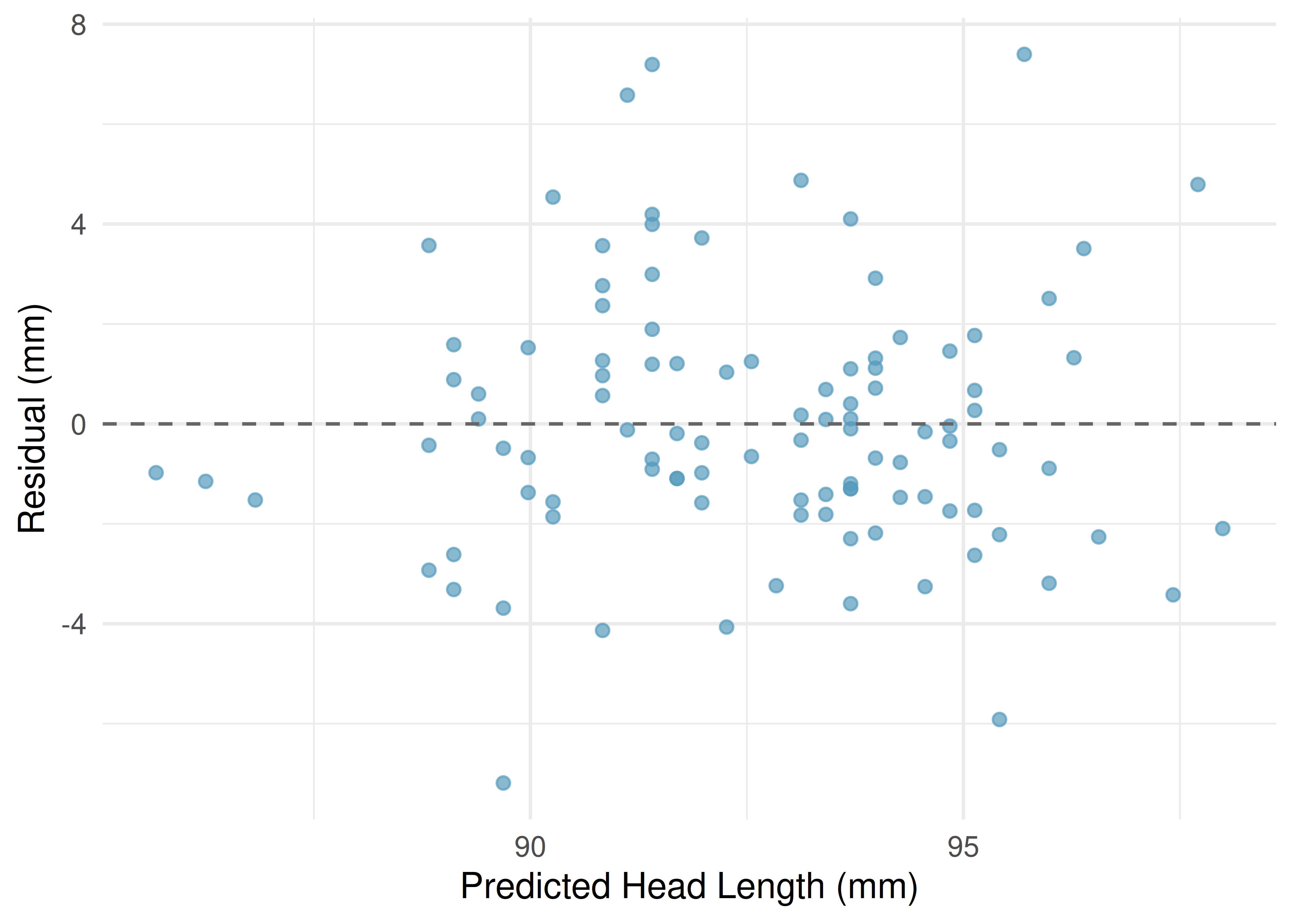
What patterns should we look for in a residual plot?
- No pattern (good): Residuals scattered randomly around zero suggest the linear model is appropriate.
- Curved pattern (bad): A U-shape or other curve in the residuals indicates a nonlinear relationship that a straight line fails to capture.
- Fan shape (bad): Increasing or decreasing spread in the residuals indicates non-constant variability.
20.3 Least squares regression
Fitting linear models by eye is subjective. Least squares regression provides an objective, rigorous approach.
20.3.1 The objective: minimize squared residuals
We want a line with small residuals. The least squares line minimizes the sum of the squared residuals:
\[e_1^2 + e_2^2 + \cdots + e_n^2\]
Why square the residuals rather than just sum their absolute values?
- It is the most commonly used method.
- It is widely supported in statistical software.
- A residual twice as large is usually more than twice as bad. Squaring accounts for this.
- The inference theory connecting the model to population parameters is most straightforward with least squares.
20.3.2 Interpreting the slope and intercept
For the Elmhurst College data, the least squares line predicting gift aid (in $1,000s) from family income (in $1,000s) is:
\[\widehat{\text{aid}} = 24.3 - 0.0431 \times \text{family\_income}\]
| Term | Estimate | Std. Error | T statistic | \(p\)-value |
|---|---|---|---|---|
| (Intercept) | 24.32 | 1.29 | 18.83 | <0.0001 |
| family_income | -0.0431 | 0.0108 | -3.98 | 0.0002 |
What do the intercept and slope mean?
Slope (\(b_1 = -0.0431\)): For each additional $1,000 of family income, we would expect a student to receive $43.10 less in gift aid, on average. The negative coefficient means higher income is associated with less aid. We must be cautious: this is an observational study, so we cannot interpret a causal connection.
Intercept (\(b_0 = 24.32\)): The model predicts that a student whose family has no income would receive $24,320 in gift aid, on average. This is meaningful because the family income for some students is near zero. In other applications, the intercept may have no practical meaning if \(x = 0\) is outside the range of the data.
Interpreting parameters estimated by least squares.
The slope describes the estimated difference in the predicted average outcome of \(y\) if the predictor variable \(x\) were one unit larger.
The intercept describes the average outcome of \(y\) if \(x = 0\), provided the linear model is valid at \(x = 0\) (which may not be the case if \(x = 0\) is far outside the observed data range).
20.3.3 Computing the slope and intercept from sample statistics
The slope can be computed using the correlation and the standard deviations of the two variables:
\[b_1 = \frac{s_y}{s_x} \cdot r\]
The least squares line always passes through the point \((\bar{x}, \bar{y})\). Using the point-slope form:
\[b_0 = \bar{y} - b_1 \cdot \bar{x}\]
Identifying the least squares line from sample statistics.
- Estimate the slope: \(b_1 = (s_y / s_x) \cdot r\).
- Find the intercept using the fact that \((\bar{x}, \bar{y})\) is on the line: \(b_0 = \bar{y} - b_1 \bar{x}\).
20.4 R-squared
We evaluated the strength of a linear relationship using \(r\). More commonly, we describe the strength of a linear fit using \(R^2\), called R-squared or the coefficient of determination.
Coefficient of determination: proportion of variability explained by the model.
\(R^2\) measures the proportion of variation in the outcome variable \(y\) that is explained by the linear model with predictor \(x\). Since \(r\) is always between \(-1\) and \(1\), \(R^2\) is always between 0 and 1.
\[R^2 = 1 - \frac{SSE}{SST}\]
where:
- \(SST = \sum (y_i - \bar{y})^2\) is the total sum of squares, measuring total variability in \(y\).
- \(SSE = \sum (y_i - \hat{y}_i)^2 = \sum e_i^2\) is the sum of squared errors, measuring leftover variability after using the model.
For simple linear regression, \(R^2 = r^2\).
For the Elmhurst data, the correlation is \(r = -0.499\). What proportion of the variability in gift aid is explained by family income?
\(R^2 = (-0.499)^2 = 0.249\), or about 25%. Family income explains about 25% of the variability in gift aid among these students.
If a linear model has a very strong negative relationship with \(r = -0.97\), how much of the variation in the outcome is explained by the predictor?
Show answer
\(R^2 = (-0.97)^2 = 0.94\), or about 94% of the variation is explained.See it in action. Two guided walkthroughs: Fit a Line by Eye lab (OLS vs. LAD losses, noise-vs-uncertainty story) and Slope Inference walkthrough (LINE conditions → \(t\)-test → interpretation). Or open the Regression Explorer or Slope \(t\)-Test directly on your own data.
20.5 Inference for the slope
We have been computing sample statistics \(b_0\) and \(b_1\), but these are estimates of population parameters \(\beta_0\) and \(\beta_1\). We now turn to formal inference: testing whether a linear relationship exists in the population.
20.5.1 Hypotheses
- \(H_0\): \(\beta_1 = 0\). There is no linear relationship between \(x\) and \(y\).
- \(H_A\): \(\beta_1 \ne 0\). There is a linear relationship between \(x\) and \(y\).
20.5.2 Randomization test for the slope
If the null hypothesis is true (\(\beta_1 = 0\)), then \(x\) and \(y\) are not linearly related. We can simulate this by permuting the response variable: randomly shuffling the \(y\) values while keeping the \(x\) values fixed. This breaks any relationship between \(x\) and \(y\).
To illustrate, we use the births14 data from the openintro R package: a random sample of 1,000 US births from 2014, with each baby’s birth weight (lbs) and length of gestation (weeks).
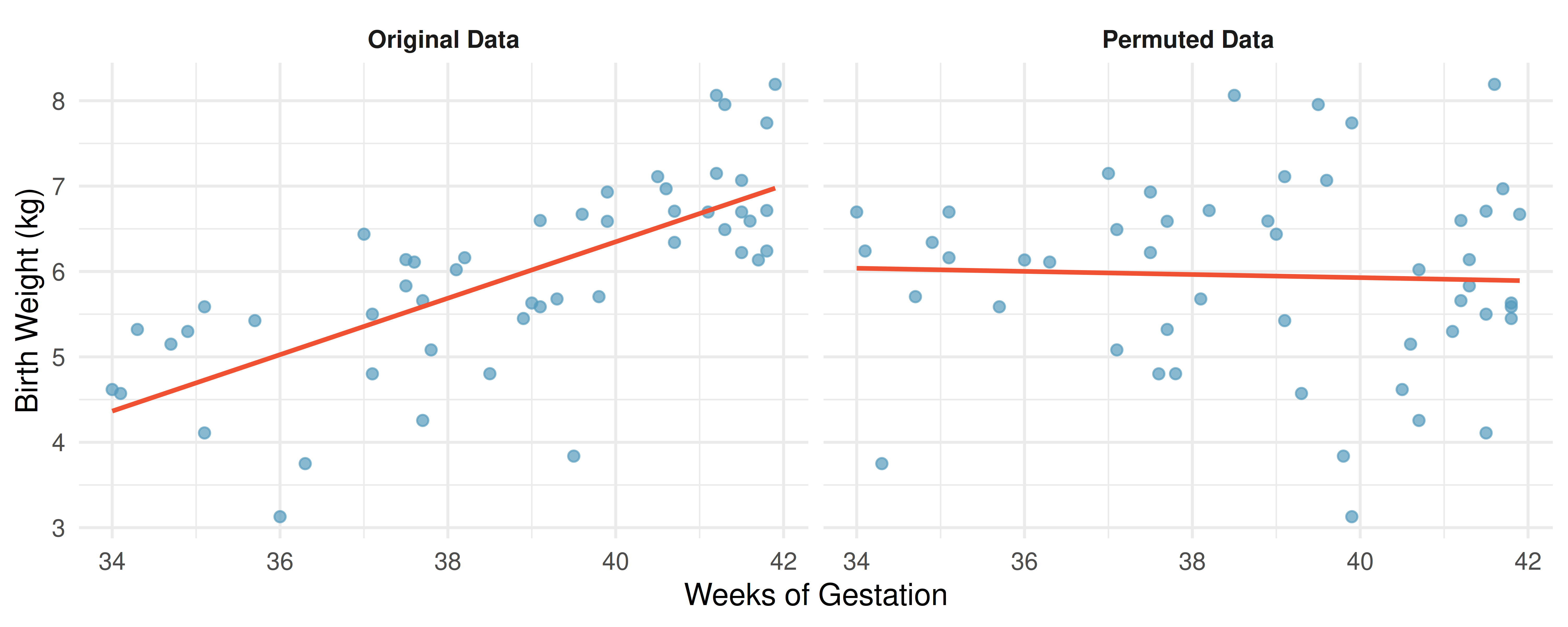
By repeating the permutation many times and computing the slope each time, we build a null distribution of slopes.
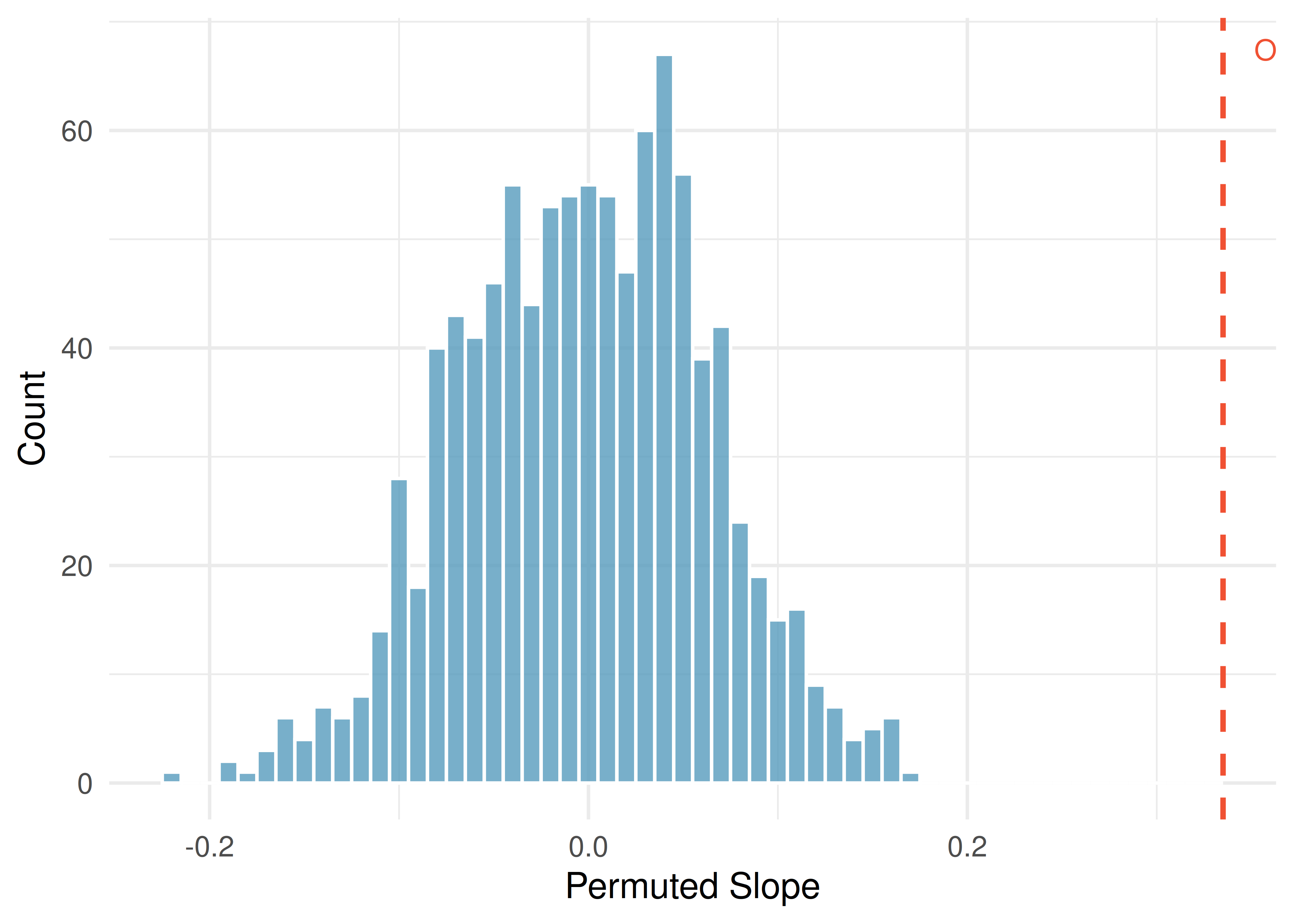
The observed slope of 0.28 lbs per week is far from any value in the null distribution. We reject \(H_0\) and conclude there is a linear relationship between weeks of gestation and birth weight.
20.5.3 Mathematical model: the t-test for slope
When the technical conditions are met, we can use the \(t\)-distribution to test the slope:
\[T = \frac{b_1 - 0}{SE_{b_1}}\]
This \(T\)-statistic follows a \(t\)-distribution with \(df = n - 2\).
The regression output for predicting the change in House seats for the President’s party from the unemployment rate is:
| Term | Estimate | Std. Error | T statistic | \(p\)-value |
|---|---|---|---|---|
| (Intercept) | -7.36 | 5.16 | -1.43 | 0.1649 |
| unemp | -0.89 | 0.835 | -1.07 | 0.2961 |
The \(p\)-value of 0.2961 is not discernible. The data do not provide convincing evidence that the unemployment rate is a useful predictor of midterm election outcomes.
20.5.4 Confidence intervals for the slope
Confidence intervals for model coefficients.
Confidence intervals for model coefficients can be computed using the \(t\)-distribution:
\[b_1 \pm t_{df}^* \times SE_{b_1}\]
where \(t_{df}^*\) is the critical value corresponding to the confidence level, with \(df = n - 2\).
Using the Elmhurst College regression output (\(b_1 = -0.0431\), \(SE = 0.0108\), \(df = 48\)), compute a 95% confidence interval for the slope.
The critical value is \(t_{48}^* = 2.01\). The confidence interval is:
\[-0.0431 \pm 2.01 \times 0.0108 = (-0.0648, -0.0214)\]
We are 95% confident that for each additional $1,000 in family income, the university’s gift aid decreases by between $21.40 and $64.80 on average.
20.6 Conditions for linear regression
For the mathematical inference to be valid, we check four conditions, often remembered by the LINE mnemonic:
- L – Linear model: The data should show a linear trend. Check the scatterplot and residual plot.
- I – Independent observations: Be cautious with time series data or clustered observations.
- N – Nearly normal residuals: Residuals should be approximately normally distributed. This is less critical for large samples (Central Limit Theorem), but outliers are always a concern.
- E – Equal variability: The variability of points around the line should be roughly constant across all values of \(x\). A “fan shape” in the residual plot indicates a violation.
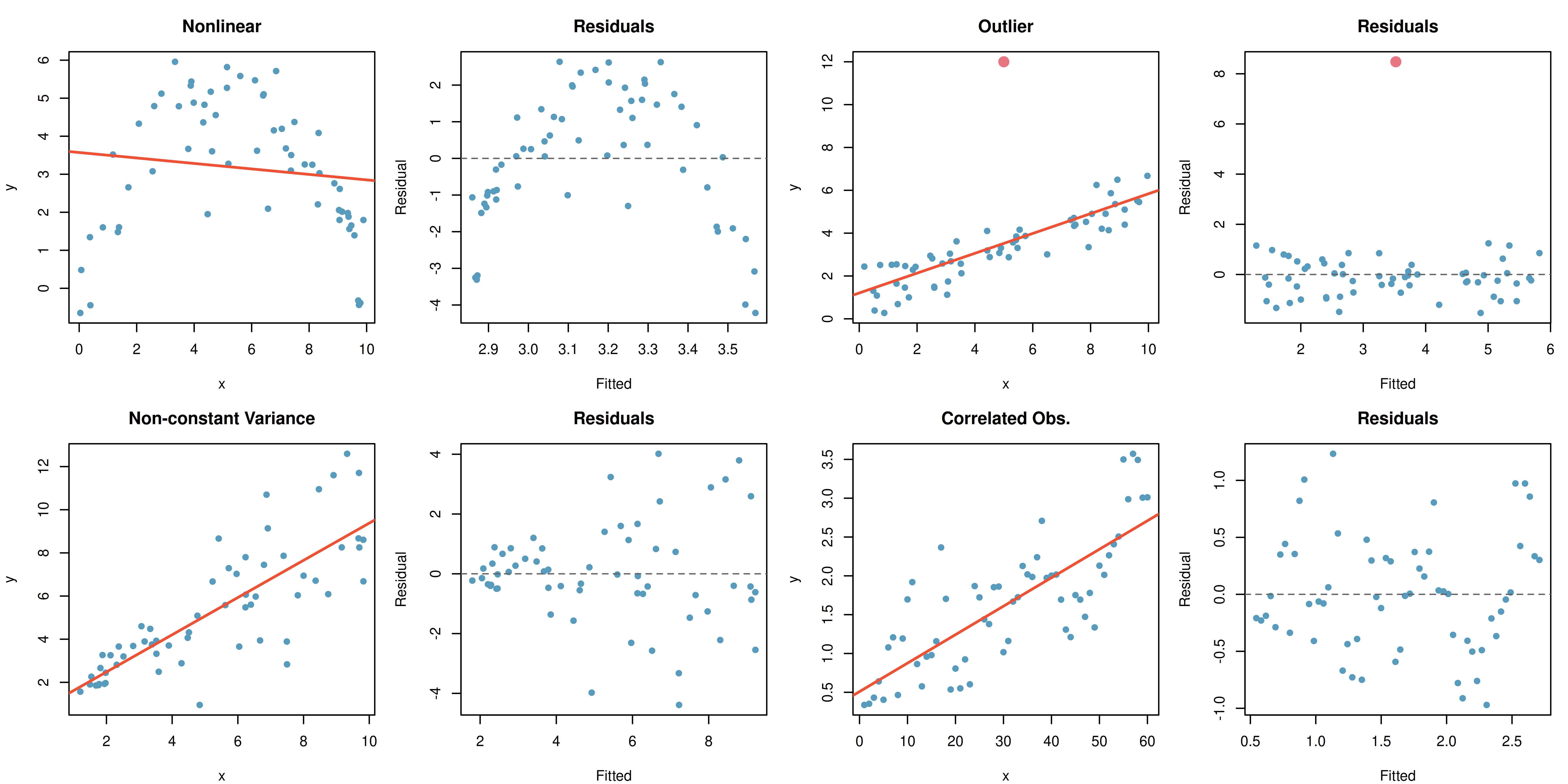
Diagnostics for linear regression.
Independence is always important. The normality condition matters most for small samples. The constant variance condition is especially important for inference. The linearity condition is the most fundamental – if the true relationship is not linear, the slope estimate has no meaningful interpretation.
20.7 Chapter review
20.7.1 Summary
In this chapter, we developed the least squares regression line as a tool for modeling the linear relationship between two quantitative variables. The slope describes the predicted change in \(y\) for a one-unit increase in \(x\), and the intercept describes the predicted value of \(y\) when \(x = 0\). Residuals measure the difference between observed and predicted values, and residual plots help assess whether the linear model is appropriate. The coefficient of determination \(R^2\) quantifies the proportion of variability in \(y\) explained by the model. For inference, we use either a randomization test or the \(t\)-distribution to test whether the slope is discernibly different from zero, and we can construct confidence intervals for the slope. The LINE conditions (linearity, independence, normality, equal variance) must be checked for the mathematical model to be valid.
20.7.2 Key terms
- Predictor / outcome variable
- Least squares line
- Slope (\(b_1\)) and intercept (\(b_0\))
- Residual
- Residual plot
- R-squared (\(R^2\)) / coefficient of determination
- Total sum of squares (SST) / sum of squared errors (SSE)
- T-test for slope
- LINE conditions
- Extrapolation
20.8 Exercises
Answers to odd-numbered exercises are provided in the Exercise Solutions appendix at the back of the book.
- Units of regression. Consider a regression predicting the number of calories (cal) from width (cm) for a sample of square shaped chocolate brownies. What are the units of the correlation coefficient, the intercept, and the slope?
- Which is higher? Determine if (I) or (II) is higher or if they are equal: “For a regression line, the uncertainty associated with the slope estimate, \(b_1\), is higher when (I) there is a lot of scatter around the regression line or (II) there is very little scatter around the regression line.” Explain your reasoning.
- The Coast Starlight, regression. The Coast Starlight Amtrak train runs from Seattle to Los Angeles. The scatterplot below displays the distance between each stop (in miles) and the amount of time it takes to travel from one stop to another (in minutes). The mean travel time from one stop to the next on the Coast Starlight is 129 mins, with a standard deviation of 113 minutes. The mean distance traveled from one stop to the next is 108 miles with a standard deviation of 99 miles. The correlation between travel time and distance is 0.636.
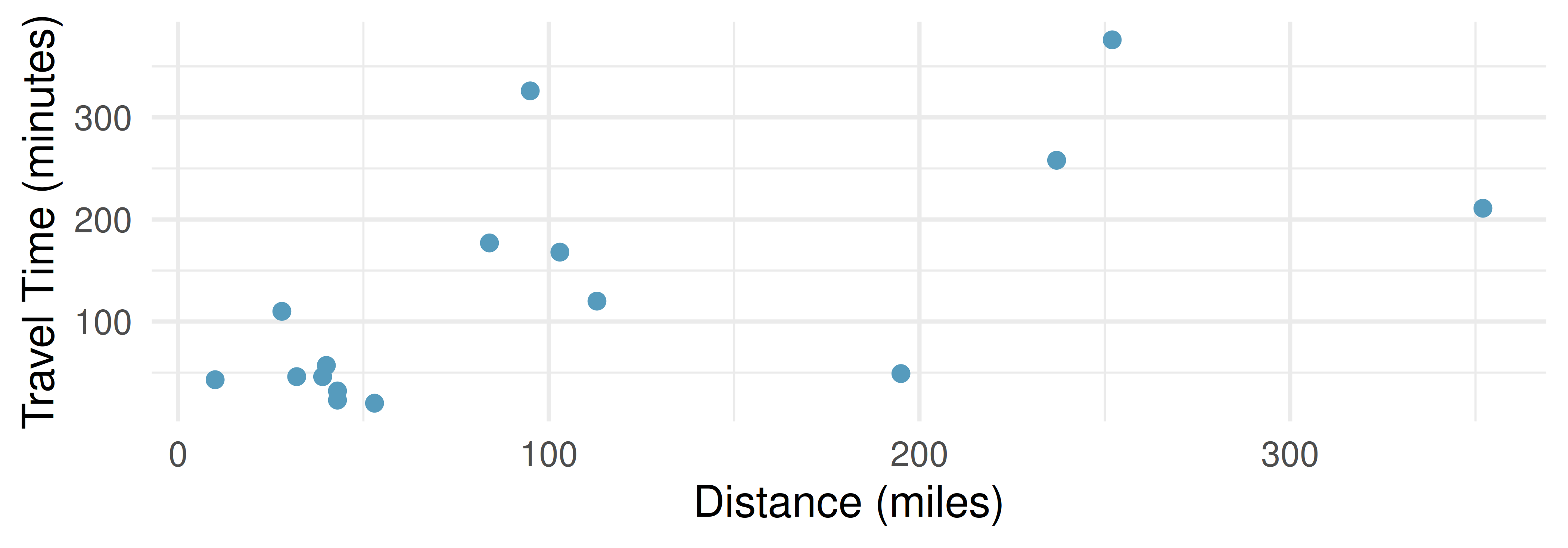
Write the equation of the regression line for predicting travel time.
Interpret the slope and the intercept in this context.
Calculate \(R^2\) of the regression line for predicting travel time from distance traveled for the Coast Starlight, and interpret \(R^2\) in the context of the application.
The distance between Santa Barbara and Los Angeles is 103 miles. Use the model to estimate the time it takes for the Starlight to travel between these two cities.
It takes the Coast Starlight about 168 mins to travel from Santa Barbara to Los Angeles. Calculate the residual and explain the meaning of this residual value.
Suppose Amtrak is considering adding a stop to the Coast Starlight 500 miles away from Los Angeles. Would it be appropriate to use this linear model to predict the travel time from Los Angeles to this point?
- Body measurements, regression. Researchers studying anthropometry collected body and skeletal diameter measurements, as well as age, weight, height and sex for 507 physically active individuals. The scatterplot below shows the relationship between height and shoulder girth (circumference of shoulders measured over deltoid muscles), both measured in centimeters. The mean shoulder girth is 107.20 cm with a standard deviation of 10.37 cm. The mean height is 171.14 cm with a standard deviation of 9.41 cm. The correlation between height and shoulder girth is 0.67. (Heinz et al. 2003)
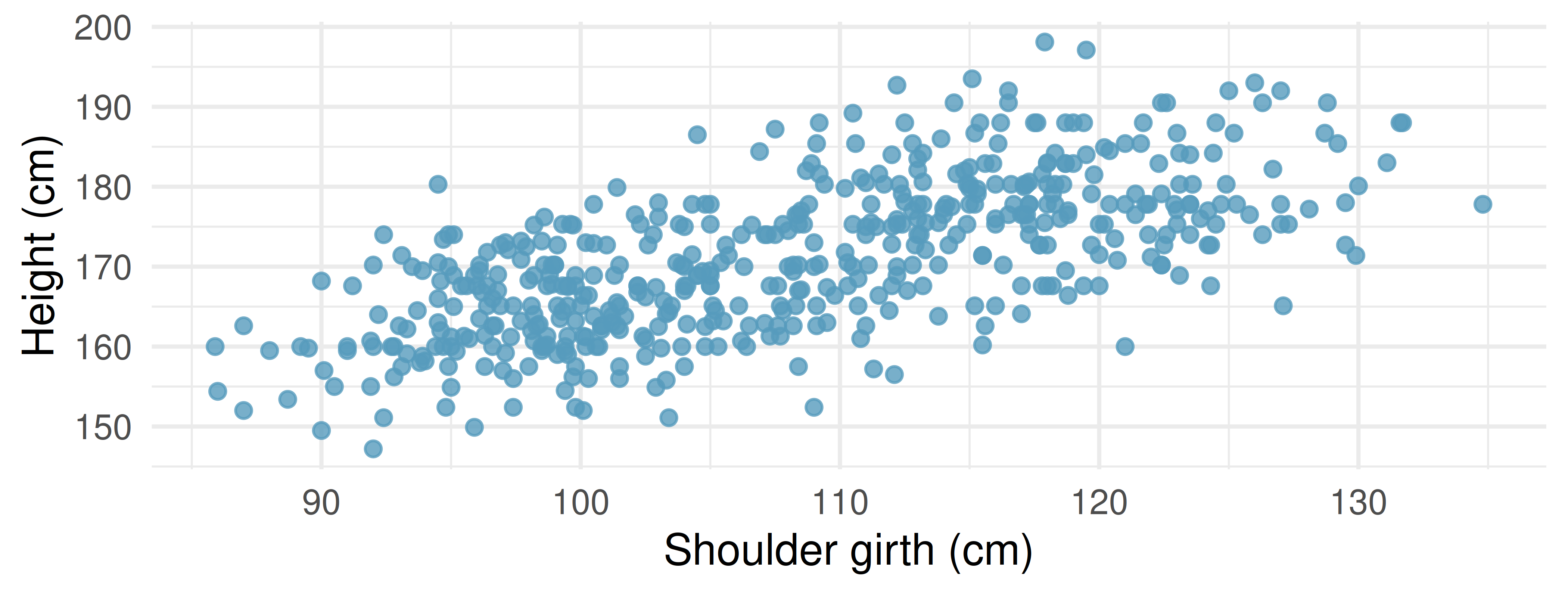
Write the equation of the regression line for predicting height.
Interpret the slope and the intercept in this context.
Calculate \(R^2\) of the regression line for predicting height from shoulder girth, and interpret it in the context of the application.
A randomly selected student from your class has a shoulder girth of 100 cm. Predict the height of this student using the model.
The student from part (d) is 160 cm tall. Calculate the residual, and explain what this residual means.
A one year old has a shoulder girth of 56 cm. Would it be appropriate to use this linear model to predict the height of this child?
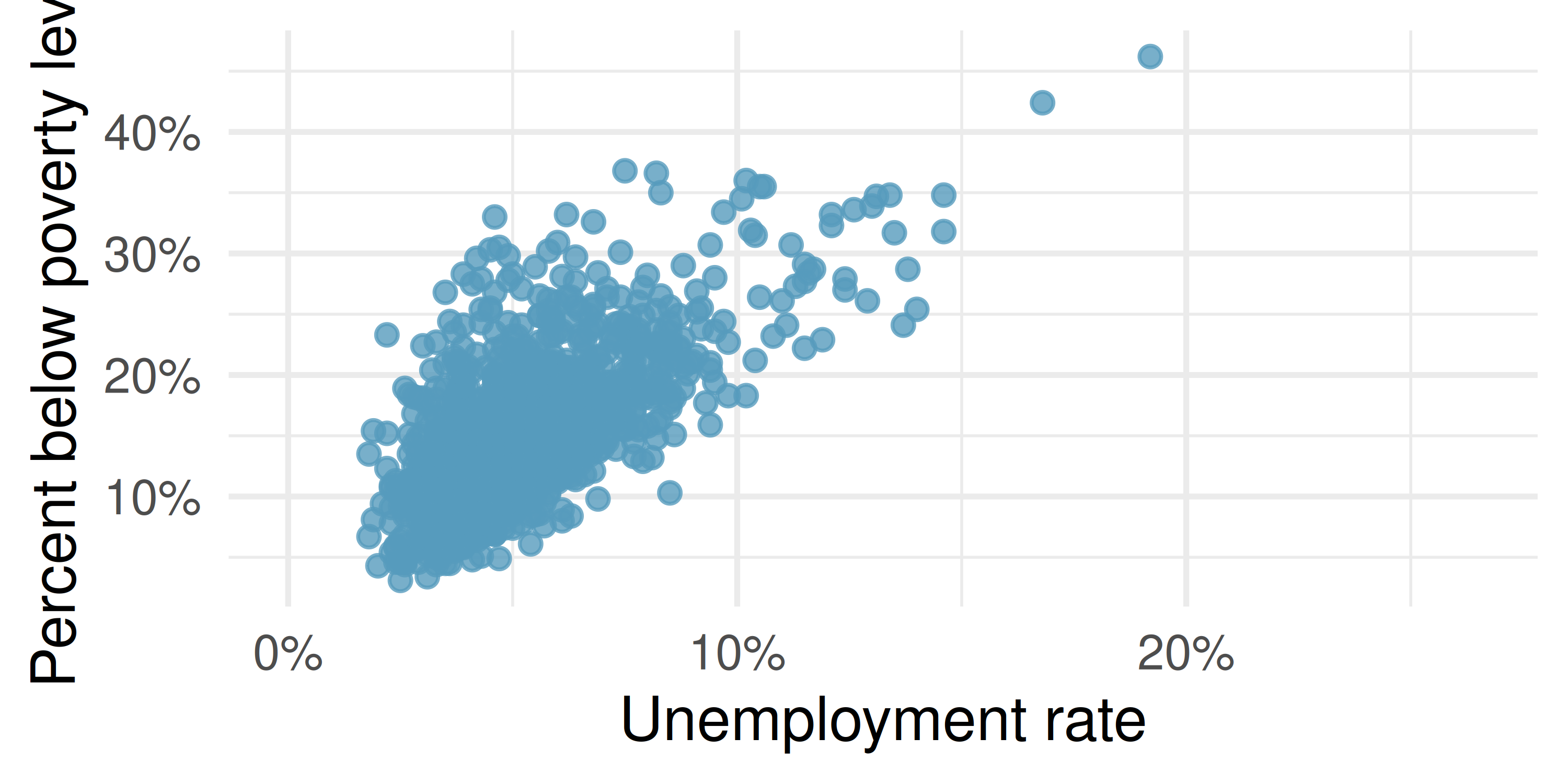
- Poverty and unemployment. The following scatterplot shows the relationship between percent of population below the poverty level (
poverty) from unemployment rate among those ages 20-64 (unemployment_rate) in counties in the US, as provided by data from the 2019 American Community Survey. The regression output for the model for predictingpovertyfromunemployment_rateis also provided.
| term | estimate | std.error | statistic | p.value |
|---|---|---|---|---|
| (Intercept) | 4.604 | 0.349 | 13.182 | <0.0001 |
| unemployment_rate | 2.054 | 0.062 | 33.110 | <0.0001 |
Write out the linear model.
Interpret the intercept.
Interpret the slope.
The \(R^2\) of this model is 46%.
Interpret this value.Calculate the correlation coefficient.
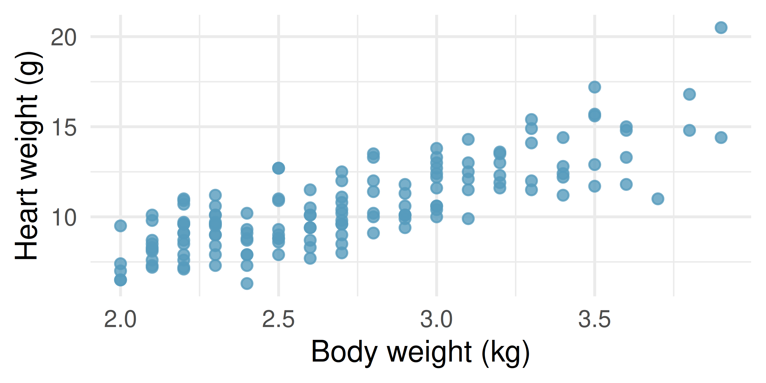
- Cat weights. The following regression output is for predicting the heart weight (
Hwt, in g) of cats from their body weight (Bwt, in kg). The coefficients are estimated using a dataset of 144 domestic cats.
| term | estimate | std.error | statistic | p.value |
|---|---|---|---|---|
| (Intercept) | -0.357 | 0.692 | -0.515 | 0.6072 |
| Bwt | 4.034 | 0.250 | 16.119 | <0.0001 |
Write out the linear model.
Interpret the intercept.
Interpret the slope.
The \(R^2\) of this model is 65%.
Interpret \(R^2\).Calculate the correlation coefficient.
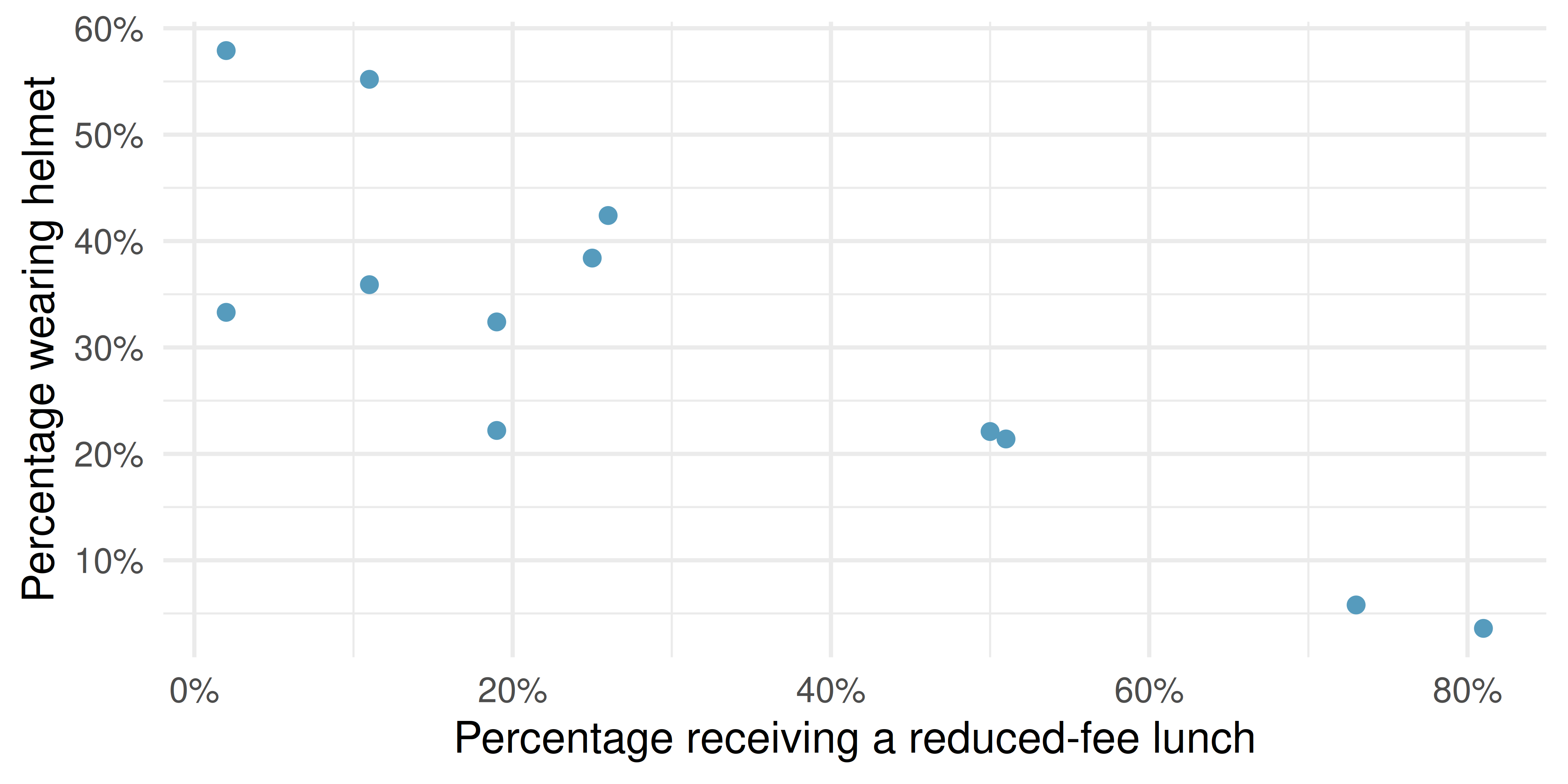
- Helmets and lunches. The scatterplot shows the relationship between socioeconomic status measured as the percentage of children in a neighborhood receiving reduced-fee lunches at school (
lunch) and the percentage of bike riders in the neighborhood wearing helmets (helmet). The average percentage of children receiving reduced-fee lunches is 30.83% with a standard deviation of 26.72% and the average percentage of bike riders wearing helmets is 30.88% with a standard deviation of 16.95%.
If the \(R^2\) for the least-squares regression line for these data is 72%, what is the correlation between
lunchandhelmet?Calculate the slope and intercept for the least-squares regression line for these data.
Interpret the intercept of the least-squares regression line in the context of the application.
Interpret the slope of the least-squares regression line in the context of the application.
What would the value of the residual be for a neighborhood where 40% of the children receive reduced-fee lunches and 40% of the bike riders wear helmets? Interpret the meaning of this residual in the context of the application.
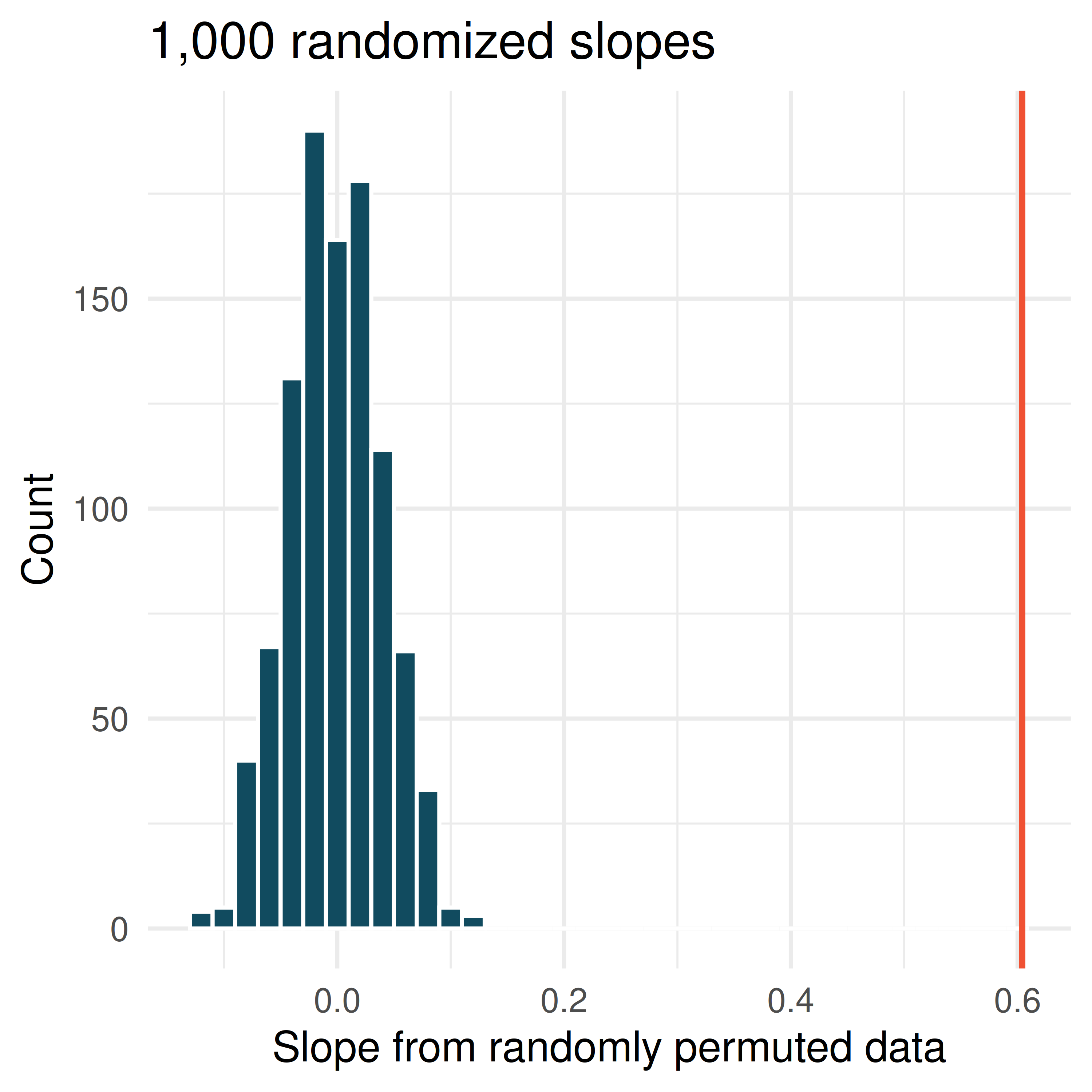
- Body measurements, randomization test. Researchers studying anthropometry collected body and skeletal diameter measurements, as well as age, weight, height and sex for 507 physically active individuals. A linear model is built to predict height based on shoulder girth (circumference of shoulders measured over deltoid muscles), both measured in centimeters. (Heinz et al. 2003) Shown below are the linear model output for predicting height from shoulder girth and the histogram of slopes from 1,000 randomized datasets (1,000 times,
hgtwas permuted and regressed againstsho_gi). The red vertical line is drawn at the observed slope value which was produced in the linear model output.
| term | estimate | std.error | statistic | p.value |
|---|---|---|---|---|
| (Intercept) | 105.832 | 3.272 | 32.340 | <0.0001 |
| sho_gi | 0.604 | 0.030 | 20.049 | <0.0001 |
What are the null and alternative hypotheses for evaluating whether the slope of the model predicting height from shoulder girth is differen than 0.
Using the histogram which describes the distribution of slopes when the null hypothesis is true, find the p-value and conclude the hypothesis test in the context of the problem (use words like shoulder girth and height).
Is the conclusion based on the histogram of randomized slopes consistent with the conclusion from the mathematical model? Explain your reasoning.
- Baby’s weight and father’s age, randomization test. US Department of Health and Human Services, Centers for Disease Control and Prevention collect information on births recorded in the country. The data used here are a random sample of 1000 births from 2014. Here, we study the relationship between the father’s age and the weight of the baby. (ICPSR 2014) Shown below are the linear model output for predicting baby’s weight (in pounds) from father’s age (in years) and the histogram of slopes from 1000 randomized datasets (1000 times,
weightwas permuted and regressed againstfage). The red vertical line is drawn at the observed slope value which was produced in the linear model output.
| term | estimate | std.error | statistic | p.value |
|---|---|---|---|---|
| (Intercept) | 7.101 | 0.199 | 35.674 | <0.0001 |
| fage | 0.005 | 0.006 | 0.757 | 0.4495 |
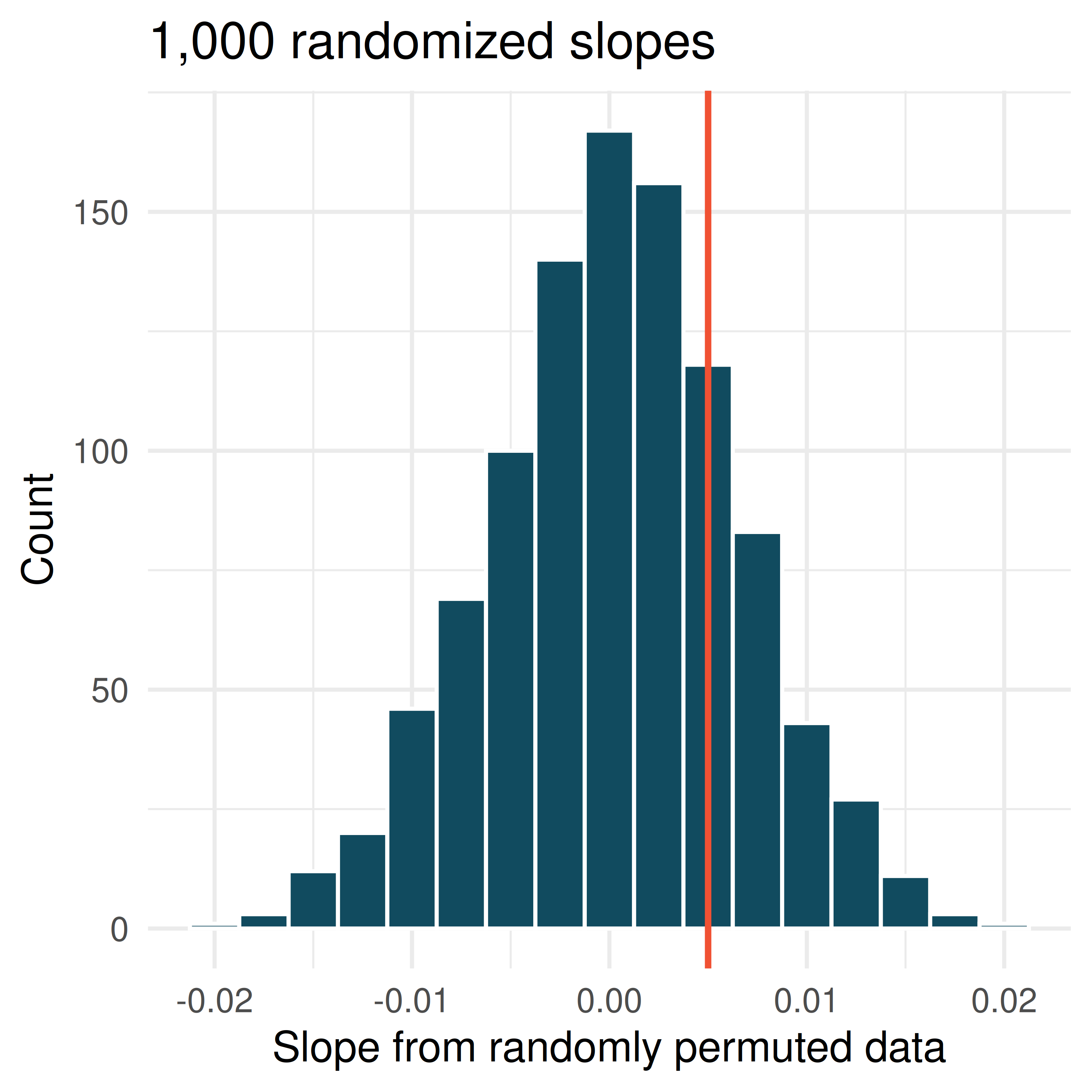
What are the null and alternative hypotheses for evaluating whether the slope of the model for predicting baby’s weight from father’s age is different than 0?
Using the histogram which describes the distribution of slopes when the null hypothesis is true, find the p-value and conclude the hypothesis test in the context of the problem (use words like father’s age and weight of baby). What does the conclusion of your test say about whether the father’s age is a useful predictor of baby’s weight?
Is the conclusion based on the histogram of randomized slopes consistent with the conclusion from the mathematical model? Explain your reasoning.
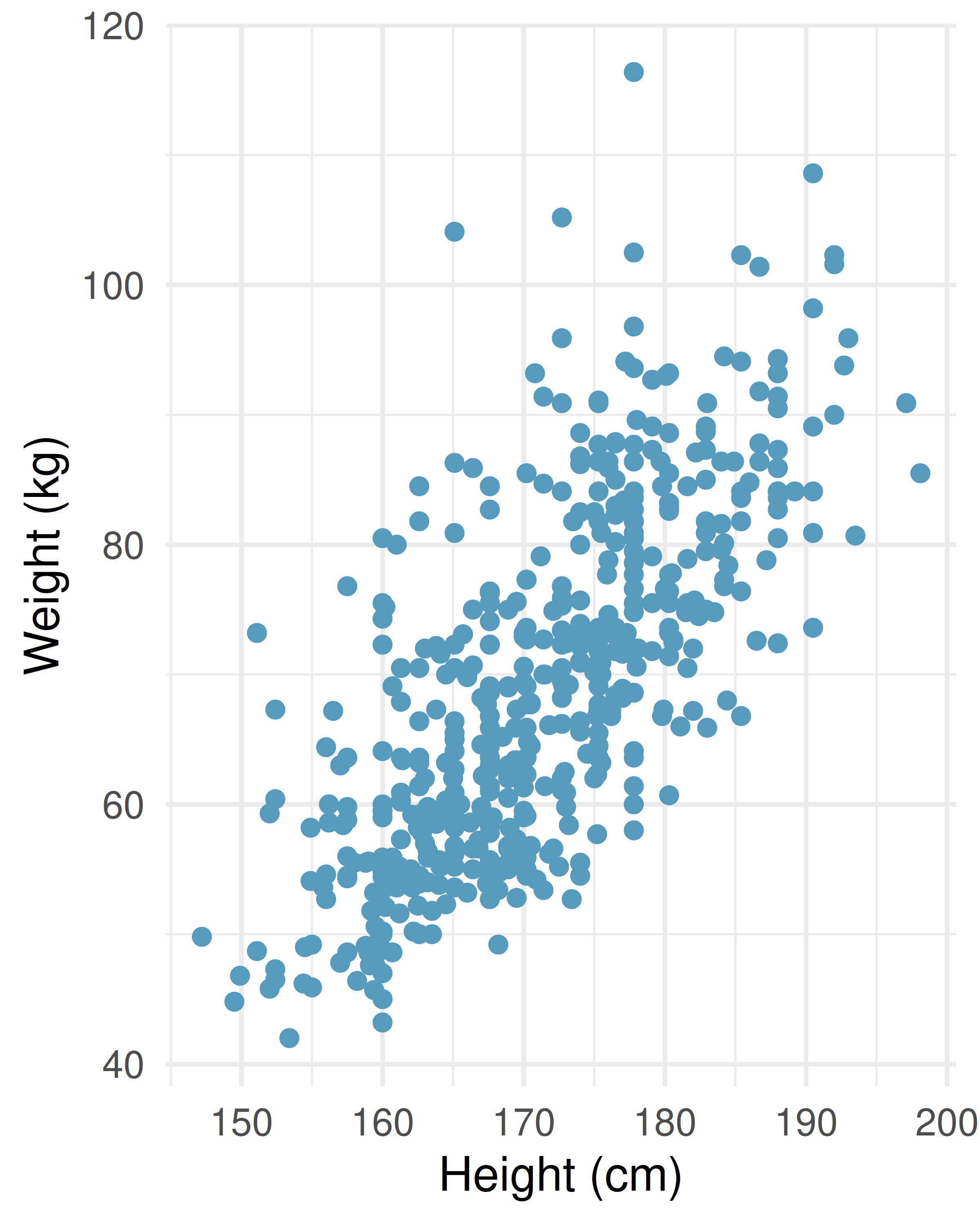
- Body measurements, mathematical test. The scatterplot and least squares summary below show the relationship between weight measured in kilograms and height measured in centimeters of 507 physically active individuals. (Heinz et al. 2003)
| term | estimate | std.error | statistic | p.value |
|---|---|---|---|---|
| (Intercept) | -105.01 | 7.54 | -13.93 | <0.0001 |
| hgt | 1.02 | 0.04 | 23.13 | <0.0001 |
Describe the relationship between height and weight.
Write the equation of the regression line. Interpret the slope and intercept in context.
Do the data provide convincing evidence that the true slope parameter is different than 0? State the null and alternative hypotheses, report the p-value (using a mathematical model), and state your conclusion.
The correlation coefficient for height and weight is 0.72. Calculate \(R^2\) and interpret it in context.
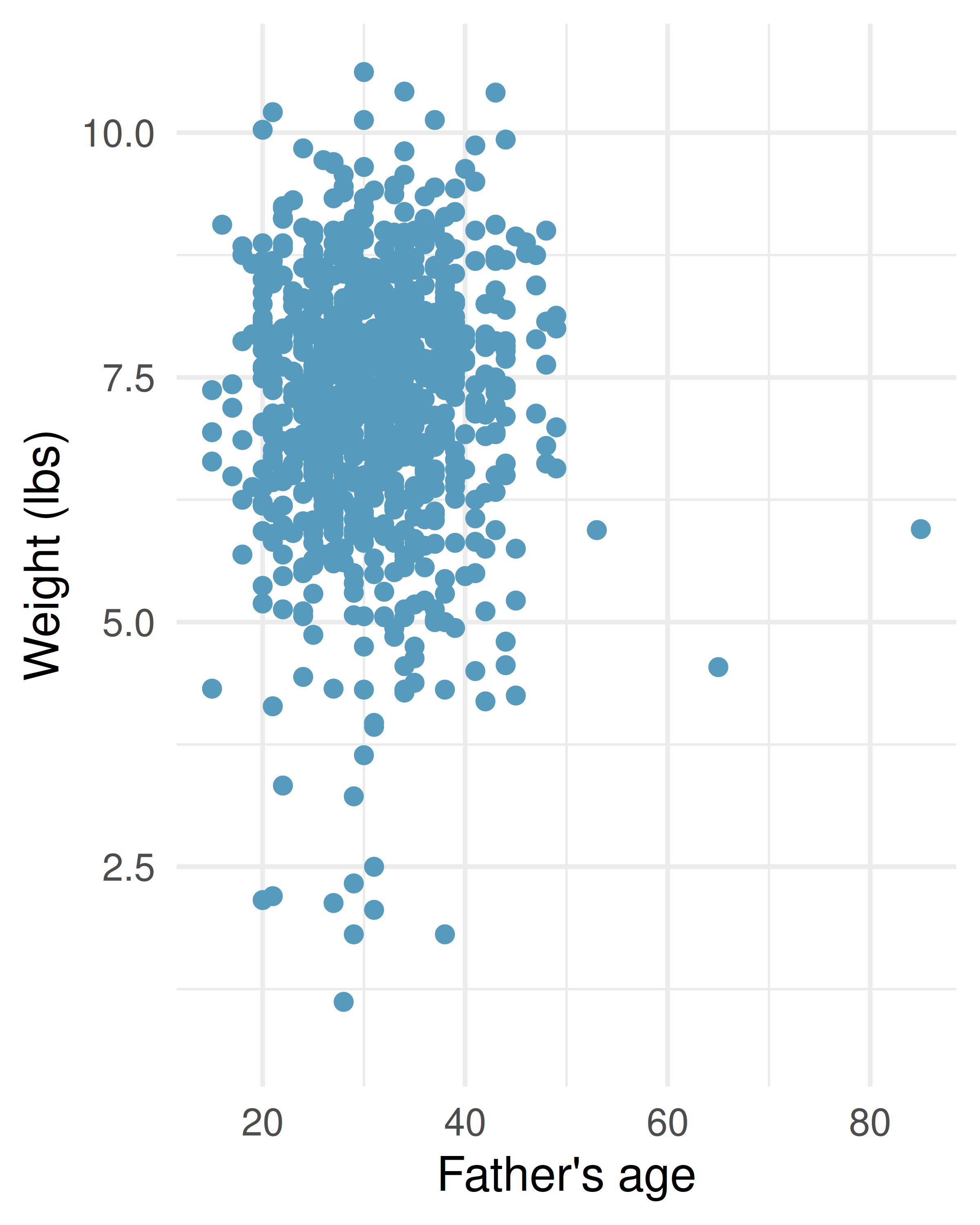
- Baby’s weight and father’s age, mathematical test. Is the father’s age useful in predicting the baby’s weight? The scatterplot and least squares summary below show the relationship between baby’s weight (measured in pounds) and father’s age for a random sample of babies. (ICPSR 2014)
| term | estimate | std.error | statistic | p.value |
|---|---|---|---|---|
| (Intercept) | 7.1042 | 0.1936 | 36.6980 | <0.0001 |
| fage | 0.0047 | 0.0061 | 0.7794 | 0.4359 |
What is the predicted weight of a baby whose father is 30 years old?
Do the data provide convincing evidence that the model for predicting baby weights from father’s age has a slope different than 0? State the null and alternative hypotheses, report the p-value (using a mathematical model), and state your conclusion.
Based on your conclusion, is father’s age a useful predictor of baby’s weight?
- Body measurements, bootstrap percentile interval. In order to estimate the slope of the model predicting height based on shoulder girth (circumference of shoulders measured over deltoid muscles), 1,000 bootstrap samples are taken from a dataset of body measurements from 507 people. A linear model predicting height based on shoulder girth is fit to each bootstrap sample, and the slope is estimated. A histogram of these slopes is shown below. (Heinz et al. 2003)
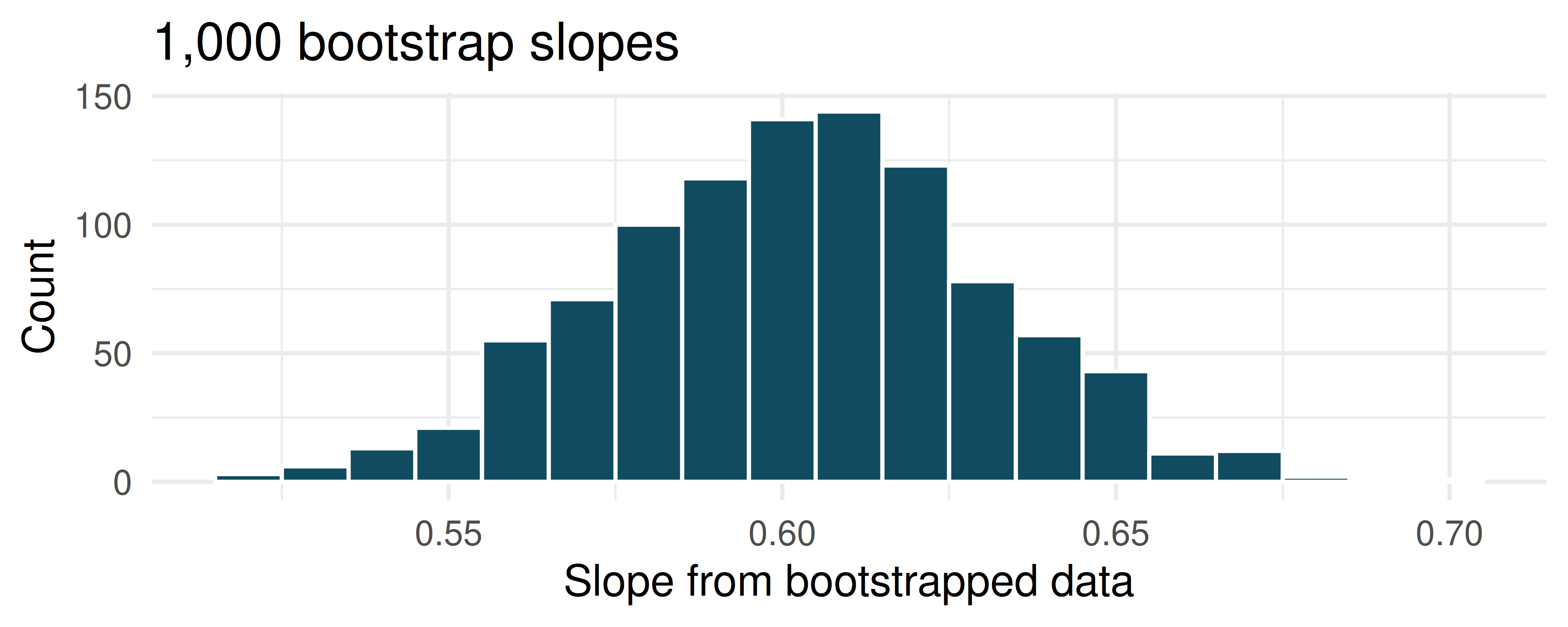
Using the bootstrap percentile method and the histogram above, find a 98% confidence interval for the slope parameter.
Interpret the confidence interval in the context of the problem.
- Baby’s weight and father’s age, bootstrap percentile interval. US Department of Health and Human Services, Centers for Disease Control and Prevention collect information on births recorded in the country. The data used here are a random sample of 1000 births from 2014. Here, we study the relationship between the father’s age and the weight of the baby. Below is the bootstrap distribution of the slope statistic from 1,000 different bootstrap samples of the data. (ICPSR 2014)
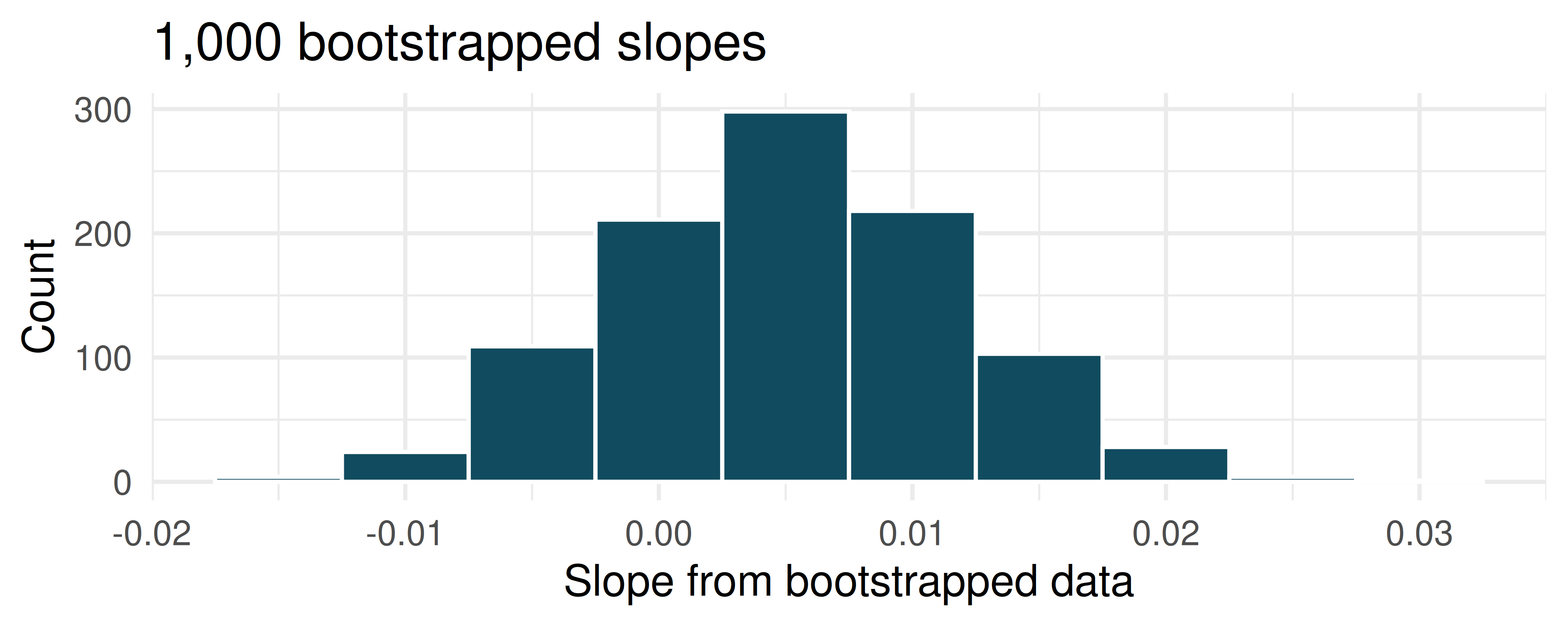
Using the bootstrap percentile method and the histogram above, find a 95% confidence interval for the slope parameter.
Interpret the confidence interval in the context of the problem.
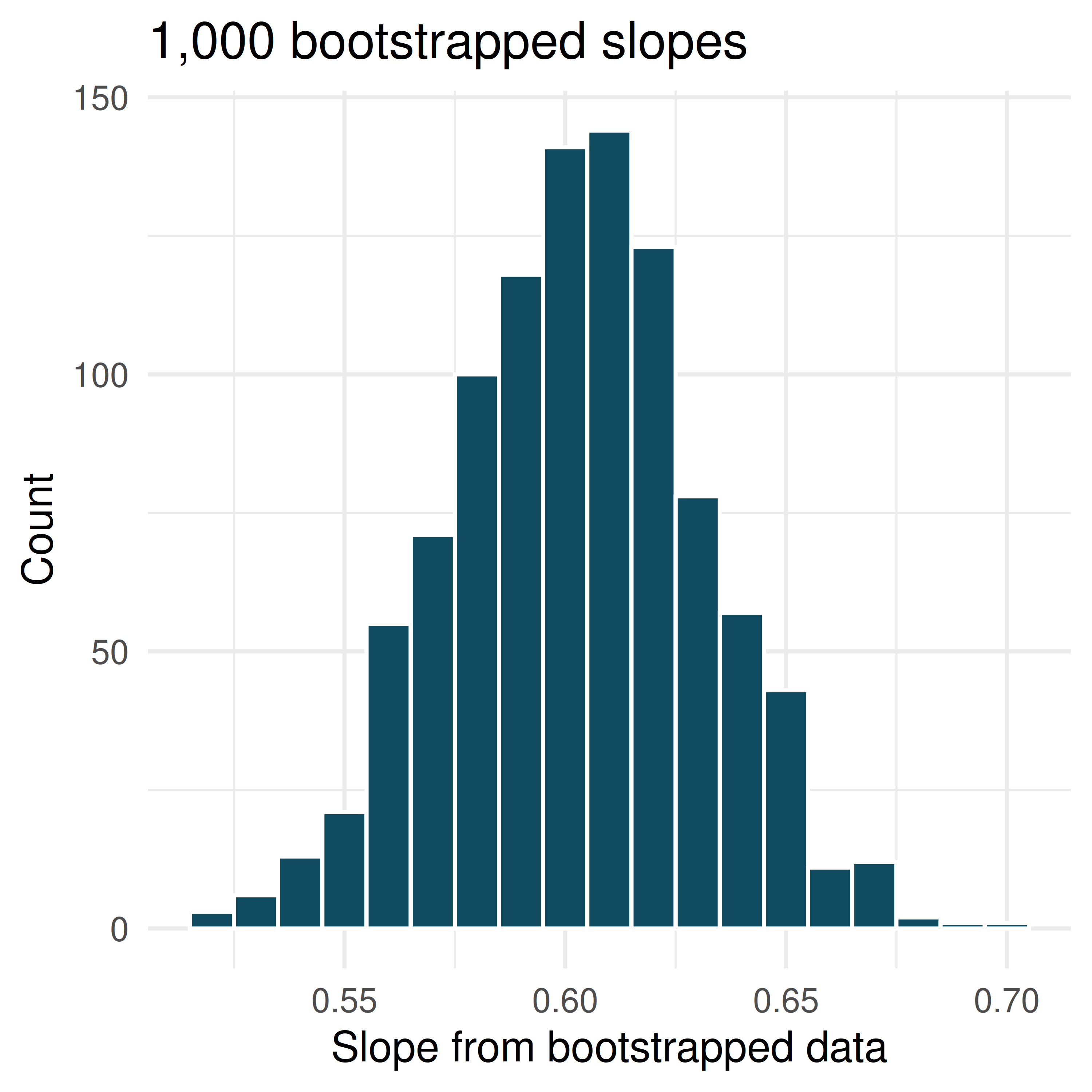
- Body measurements, standard error bootstrap interval. A linear model is built to predict height based on shoulder girth (circumference of shoulders measured over deltoid muscles), both measured in centimeters. (Heinz et al. 2003) Shown below are the linear model output for predicting height from shoulder girth and the bootstrap distribution of the slope statistic from 1,000 different bootstrap samples of the data.
| term | estimate | std.error | statistic | p.value |
|---|---|---|---|---|
| (Intercept) | 105.832 | 3.272 | 32.340 | <0.0001 |
| sho_gi | 0.604 | 0.030 | 20.049 | <0.0001 |
Using the histogram, approximate the standard error of the slope statistic (that is, quantify the variability of the slope statistic from sample to sample).
Find a 98% bootstrap SE confidence interval for the slope parameter.
Interpret the confidence interval in the context of the problem.
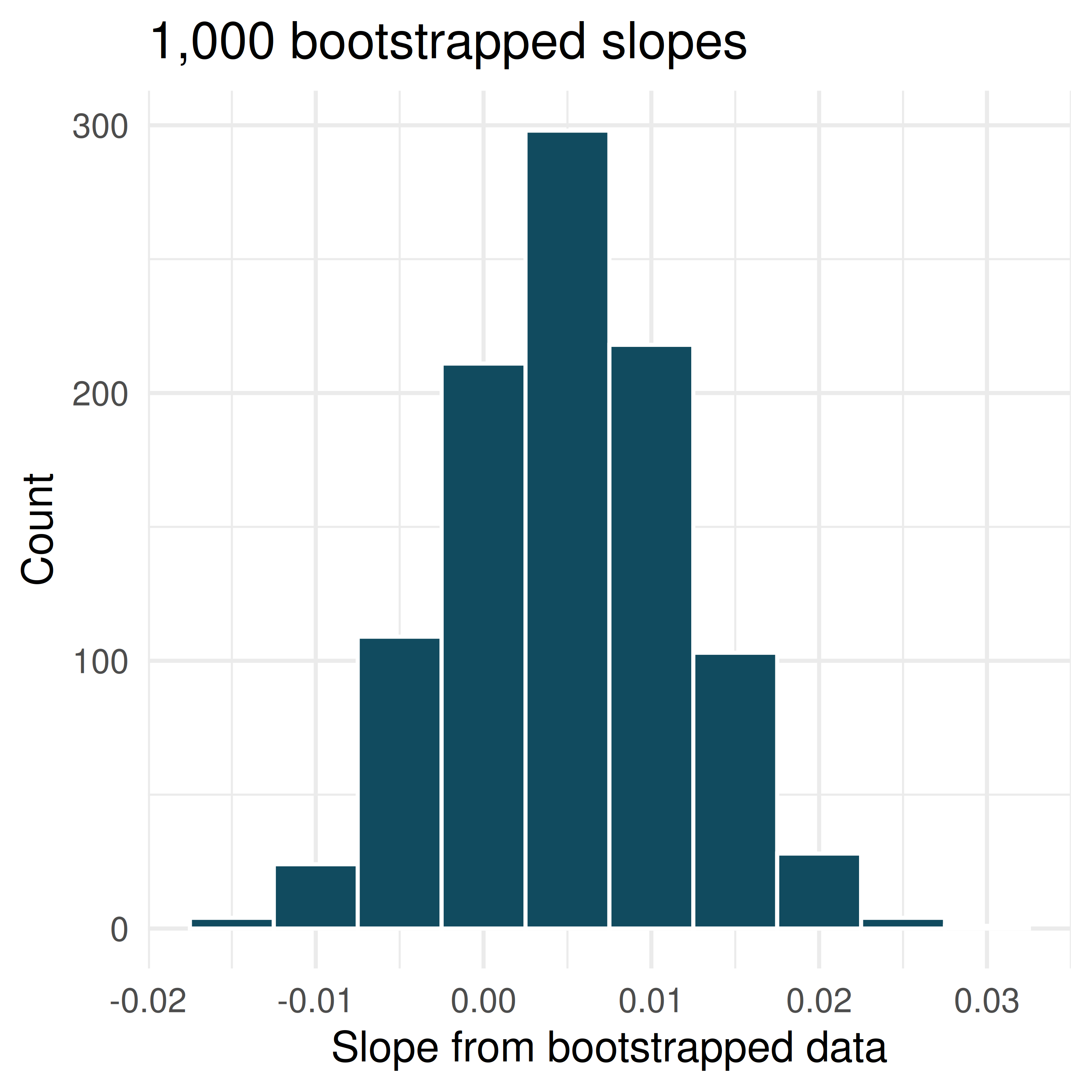
- Baby’s weight and father’s age, standard error bootstrap interval. US Department of Health and Human Services, Centers for Disease Control and Prevention collect information on births recorded in the country. The data used here are a random sample of 1000 births from 2014. Here, we study the relationship between the father’s age and the weight of the baby. (ICPSR 2014) Shown below are the linear model output for predicting baby’s weight (in pounds) from father’s age (in years) and the the bootstrap distribution of the slope statistic from 1000 different bootstrap samples of the data.
| term | estimate | std.error | statistic | p.value |
|---|---|---|---|---|
| (Intercept) | 7.101 | 0.199 | 35.674 | <0.0001 |
| fage | 0.005 | 0.006 | 0.757 | 0.4495 |
Using the histogram, approximate the standard error of the slope statistic (that is, quantify the variability of the slope statistic from sample to sample).
Find a 95% bootstrap SE confidence interval for the slope parameter.
Interpret the confidence interval in the context of the problem.
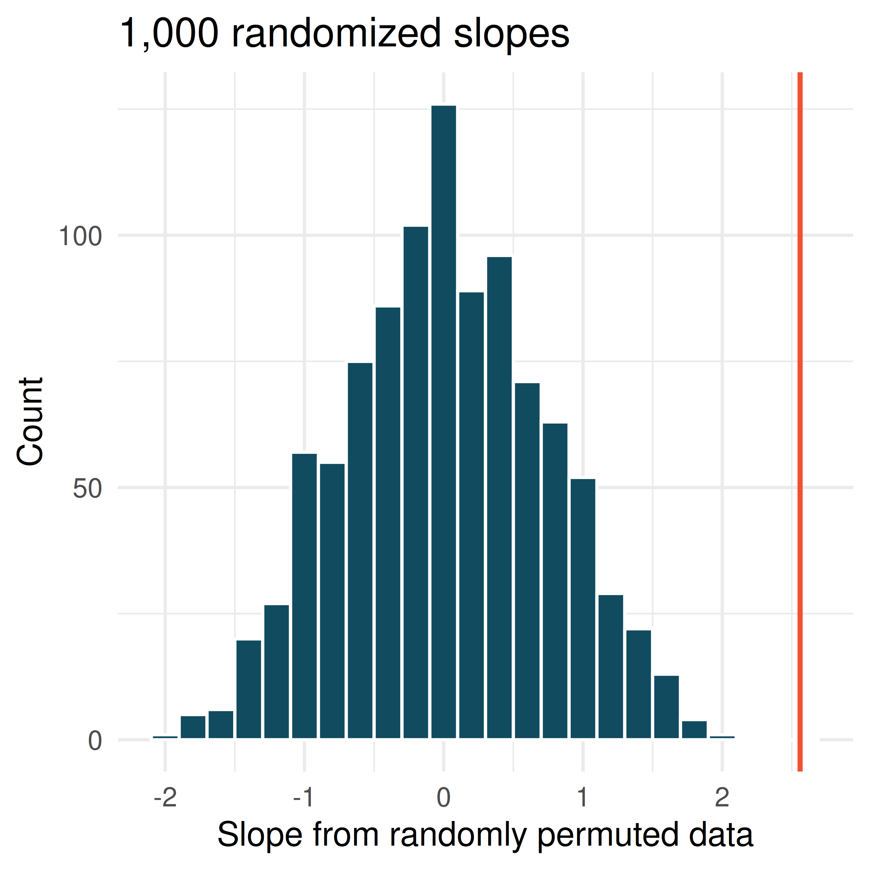
- Murders and poverty, randomization test. The following regression output is for predicting annual murders per million (
annual_murders_per_mil) from percentage living in poverty (perc_pov) in a random sample of 20 metropolitan areas. Shown below are the linear model output for predicting annual murders per million from percentage living in poverty for metropolitan areas and the histogram of slopes from 1000 randomized datasets (1000 times,annual_murders_per_milwas permuted and regressed againstperc_pov). The red vertical line is drawn at the observed slope value which was produced in the linear model output.
| term | estimate | std.error | statistic | p.value |
|---|---|---|---|---|
| (Intercept) | -29.901 | 7.789 | -3.839 | 0.0012 |
| perc_pov | 2.559 | 0.390 | 6.562 | <0.0001 |
What are the null and alternative hypotheses for evaluating whether the slope of the model for predicting annual murder rate from poverty percentage is different than 0?
Using the histogram which describes the distribution of slopes when the null hypothesis is true, find the p-value and conclude the hypothesis test in the context of the problem (use words like murder rate and poverty).
Is the conclusion based on the histogram of randomized slopes consistent with the conclusion which would have been obtained using the mathematical model? Explain your reasoning.
- Murders and poverty, mathematical test. The table below shows the output of a linear model annual murders per million (
annual_murders_per_mil) from percentage living in poverty (perc_pov) in a random sample of 20 metropolitan areas.
| term | estimate | std.error | statistic | p.value |
|---|---|---|---|---|
| (Intercept) | -29.9012 | 7.7892 | -3.8388 | 0.0012 |
| perc_pov | 2.5594 | 0.3900 | 6.5623 | <0.0001 |
What are the hypotheses for evaluating whether the slope of the model predicting annual murder rate from poverty percentage is different than 0?
State the conclusion of the hypothesis test from part (a) in context. What does this say about whether poverty percentage is a useful predictor of annual murder rate?
Calculate a 95% confidence interval for the slope of poverty percentage, and interpret it in context.
Do your results from the hypothesis test and the confidence interval agree? Explain your reasoning.
- Murders and poverty, bootstrap percentile interval. Data on annual murders per million (
annual_murders_per_mil) and percentage living in poverty (perc_pov) is collected from a random sample of 20 metropolitan areas. Using these data we want to estimate the slope of the model predictingannual_murders_per_milfromperc_pov. We take 1,000 bootstrap samples of the data and fit a linear model predictingannual_murders_per_milfromperc_povto each bootstrap sample. A histogram of these slopes is shown below.
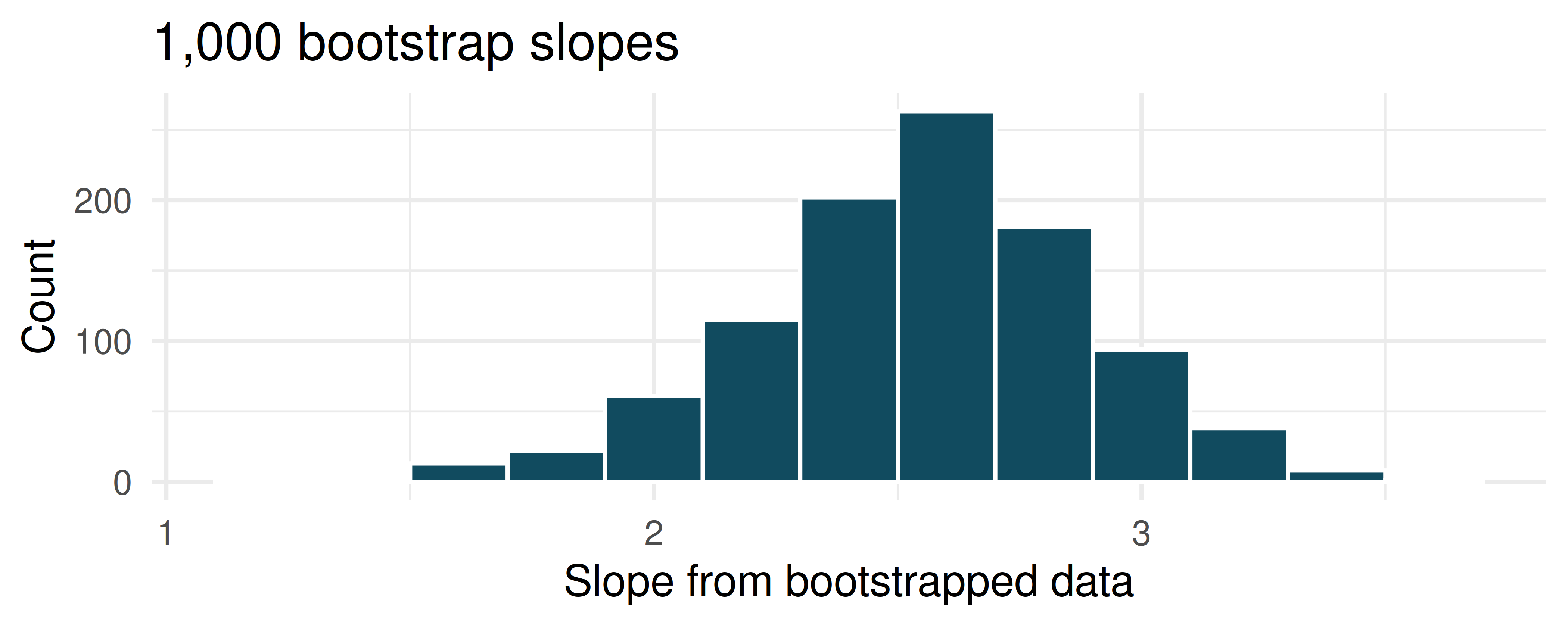
Using the percentile bootstrap method and the histogram above, find a 90% confidence interval for the slope parameter.
Interpret the confidence interval in the context of the problem.
- Murders and poverty, standard error bootstrap interval. A linear model is built to predict annual murders per million (
annual_murders_per_mil) from percentage living in poverty (perc_pov) in a random sample of 20 metropolitan areas. Shown below are the standard linear model output for predicting annual murders per million from percentage living in poverty for metropolitan areas and the bootstrap distribution of the slope statistic from 1000 different bootstrap samples of the data.
| term | estimate | std.error | statistic | p.value |
|---|---|---|---|---|
| (Intercept) | -29.901 | 7.789 | -3.839 | 0.0012 |
| perc_pov | 2.559 | 0.390 | 6.562 | <0.0001 |
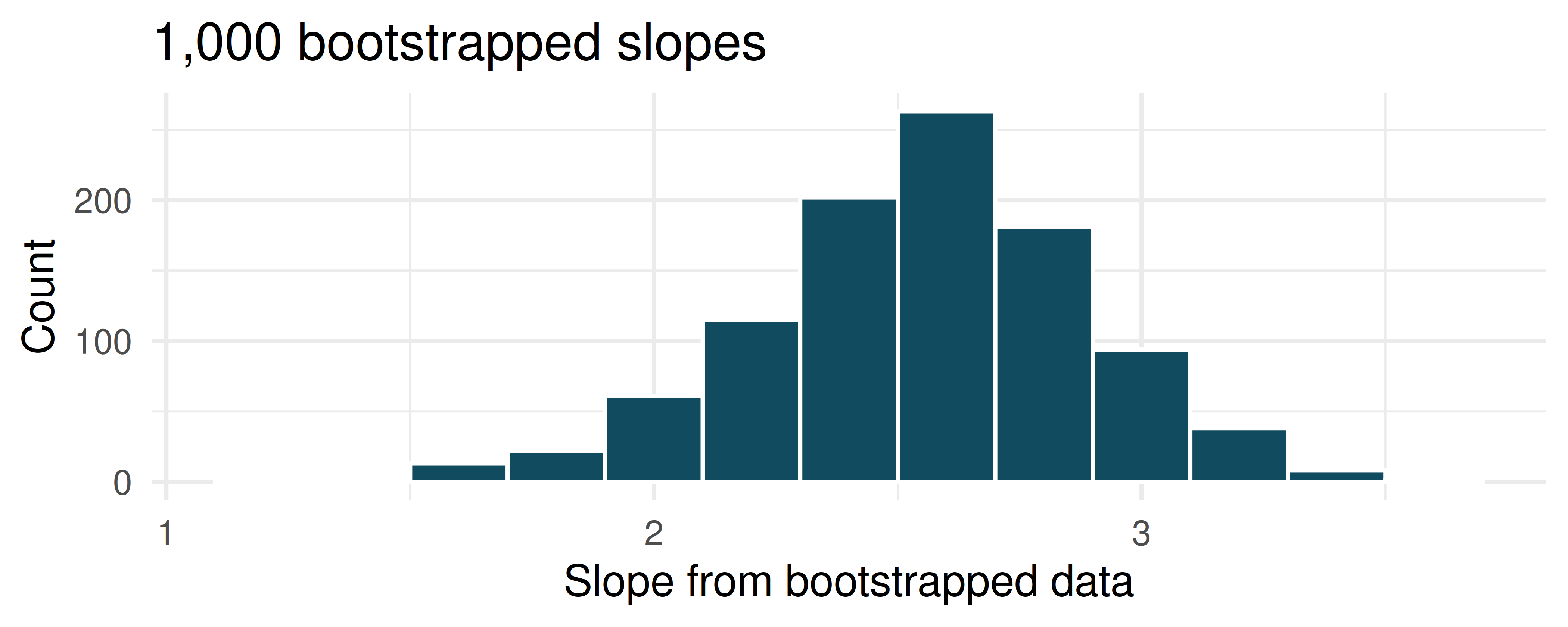
Using the histogram, approximate the standard error of the slope statistic (that is, quantify the variability of the slope statistic from sample to sample).
Find a 90% bootstrap SE confidence interval for the slope parameter.
Interpret the confidence interval in the context of the problem.
- I heart cats. Researchers collected data on heart and body weights of 144 domestic adult cats. The table below shows the output of a linear model predicting heart weight (measured in grams) from body weight (measured in kilograms) of these cats.
| term | estimate | std.error | statistic | p.value |
|---|---|---|---|---|
| (Intercept) | -0.3567 | 0.6923 | -0.5152 | 0.6072 |
| Bwt | 4.0341 | 0.2503 | 16.1194 | <0.0001 |
What are the hypotheses for evaluating whether body weight is positively associated with heart weight in cats?
State the conclusion of the hypothesis test from part (a) in context.
Calculate a 95% confidence interval for the slope of body weight, and interpret it in context.
Do your results from the hypothesis test and the confidence interval agree? Explain your reasoning.
- Beer and blood alcohol content. Many people believe that weight, drinking habits, and many other factors are much more important in predicting blood alcohol content (BAC) than simply considering the number of drinks a person consumed. Here we examine data from sixteen student volunteers at Ohio State University who each drank a randomly assigned number of cans of beer. These students were evenly divided between men and women, and they differed in weight and drinking habits. Thirty minutes later, a police officer measured their blood alcohol content (BAC) in grams of alcohol per deciliter of blood. The scatterplot and regression table summarize the findings. (Malkevitch and Lesser 2008)
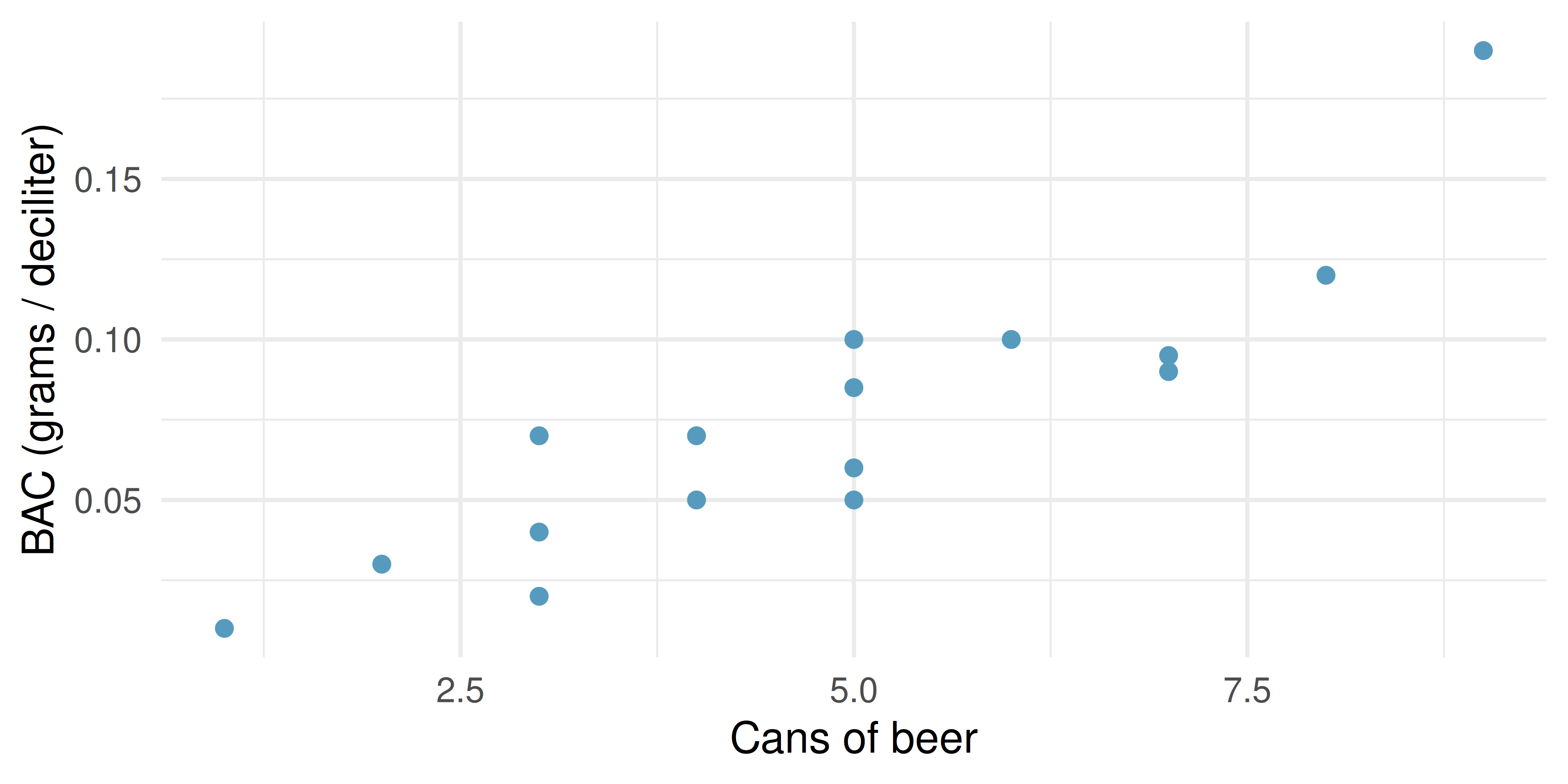
| term | estimate | std.error | statistic | p.value |
|---|---|---|---|---|
| (Intercept) | -0.0127 | 0.0126 | -1.0050 | 0.332 |
| beers | 0.0180 | 0.0024 | 7.4796 | <0.0001 |
Describe the relationship between the number of cans of beer and BAC.
Write the equation of the regression line. Interpret the slope and intercept in context.
Do the data provide convincing evidence that drinking more cans of beer is associated with an increase in blood alcohol? State the null and alternative hypotheses, report the p-value, and state your conclusion.
The correlation coefficient for number of cans of beer and BAC is 0.89. Calculate \(R^2\) and interpret it in context.
Suppose we visit a bar in our own town, ask people how many drinks they have had, and also measure their BAC. Would the relationship between number of drinks and BAC would be as strong as the relationship found in the Ohio State study? Why?
Dataset sources
coast_starlight (openintro) | bdims (openintro) | county_2019 (usdata) | cats (MASS) | births14 (openintro) | cats (MASS) | bac (openintro)
StatLens Exercises
These exercises focus on the parts of regression inference a calculator can’t do for you: framing the question, choosing the right procedure, checking the four regression conditions, and interpreting slopes and intervals without falling into the standard traps. Let StatLens do the arithmetic.
Frame the question. A real-estate analyst fits a simple linear regression of house price (response, \(\$1000\text{s}\)) on square footage (explanatory) using 200 homes in one zip code. The fitted line is \(\widehat{\text{price}} = 80 + 0.15 \cdot \text{sqft}\).
- Identify the explanatory and response variables and give the symbol for the population slope.
- Write the null and alternative hypotheses for a two-sided test of whether square footage is associated with price.
- The slope is 0.15. Interpret it in context, including units. Then identify the most common error students make in slope interpretation.
Choose the procedure. For each scenario, name the procedure — CI for slope \(\beta_1\), hypothesis test for \(\beta_1\), correlation test (\(\rho = 0\)), or not a regression problem.
- Is there evidence of any linear association between hours studied and exam score?
- Estimate, with a margin of error, how much exam score changes per extra hour studied.
- Compare the mean exam score in morning vs. evening sections of the same course.
- Decide whether the strength of the linear relationship between two variables is statistically discernible from zero.
- Estimate the mean weight of all puppies in a litter from a sample of 8.
Check the conditions before you trust the slope. Open a regression dataset in the Regression Slope tool; pair it with the Regression scatterplot for diagnostics.
- Name the four regression conditions (often summarized as “LINE”: Linearity, Independence, Normality of residuals, Equal variance of residuals).
- Open the residual plot. What pattern in the residuals would convince you that the linearity condition has failed? What pattern would convince you the equal-variance condition has failed?
- Suppose one observation has a residual five times larger than any other. Should you discard it before re-running the regression? What two questions should you ask first?
Run it and interpret it. Open any regression dataset in the Regression Slope tool.
Report the estimated slope \(b_1\), its standard error, the \(t\) statistic, and the p-value.
Read off the 95% confidence interval for \(\beta_1\). Does it contain 0?
Write a one-sentence conclusion in context, naming both variables, the direction, and the strength of evidence.
Which statement is the correct interpretation of the 95% CI for \(\beta_1\)?
- There is a 95% probability that the true slope lies in this interval.
- If the study were repeated many times, about 95% of the intervals built this way would contain the true slope.
- 95% of the data points fall within this interval.
- About 95% of the predicted responses fall within this interval.
Simulation vs. analytic — the bootstrap slope as a check. The \(t\)-CI for the slope (\(b_1 \pm t^* \cdot \text{SE}(b_1)\)) assumes the LINE conditions hold. The bootstrap CI for the slope assumes only that the data are an i.i.d. sample from the population. You will compare them.
First a well-behaved case. Open any roughly linear, homoscedastic regression dataset in both the Regression Slope tool and the Bootstrap Slope tool (generate 5000 resamples in the latter).
- Compare the two 95% intervals for \(\beta_1\). How close are they?
Now a troublesome case. Pick a regression dataset (or paste in one) with visible heteroscedasticity — a clear fan-shaped residual pattern.
- Compare the two 95% intervals again. Do they still agree? Which one is wider?
- Explain the pattern. The bootstrap resamples whole \((x, y)\) pairs, so it “sees” the heteroscedasticity — the resampled slopes fluctuate more in some parts of \(x\) than others. The \(t\)-formula uses a single SE pooled across all \(x\), which under-counts the variability in the high-spread region. Which interval is more honest?
- A student concludes: “If the conditions fail, you must transform the data.” Why is that the first impulse, but not the only one? When is the bootstrap CI the better tool even after a transformation?
Heinz, G., L. J. Peterson, R. W. Johnson, and C. J. Kerk. 2003. “Exploring Relationships in Body Dimensions.” Journal of Statistics Education 11 (2). http://www.openintro.org/redirect.php?go=textbook-body_dim_2003.
ICPSR. 2014. “United States Department of Health and Human Services. Centers for Disease Control and Prevention. National Center for Health Statistics. Natality Detail File, 2014 United States. Inter-University Consortium for Political and Social Research, 2016-10-07.” https://doi.org/10.3886/ICPSR36461.v1.
Malkevitch, J., and L. M. Lesser. 2008. For All Practical Purposes: Mathematical Literacy in Today’s World. WH Freeman & Co.