6  Sampling Variability

So far in this course, you have learned how to collect data, visualize it, and compute summary statistics. But statistics is about more than describing the data you have — it is about using data to learn about a larger population. The central challenge is this: every sample is different. If you took another sample from the same population, you would get different results. This chapter introduces the foundational ideas that make statistical inference possible: the distinction between parameters and statistics, the concept of a sampling distribution, and the standard error as a measure of how much sample statistics vary. These ideas are the bridge from describing data to drawing conclusions about the world.

Two quick warmups: how good is your intuition about randomness?

• Are You Psychic? — predict a series of coin flips, see your score, then watch the tool simulate hundreds of random guessers. How impressive is your result compared to pure chance?
• Stump the Chump — type an H/T sequence you think “looks random,” then compare it to a truly random sequence. Run lengths, alternation rates, and the longest run will tell you whether human-generated “randomness” is too even.

Both are short interactive demos that motivate the rest of this chapter: real random samples vary more than people expect, and that variability has a predictable shape.

6.1 Parameters vs. statistics

When we collect data, we typically have a larger group in mind. A political poll surveys 1,000 likely voters, but the real interest is in all voters. A quality engineer measures 50 widgets from an assembly line, but the real interest is in all widgets the line produces. The larger group is the population; the subset we actually observe is the sample.

A population parameter is a numerical summary of the entire population. It is a fixed number, but it is almost always unknown because we cannot observe the whole population.

A sample statistic (also called a point estimate) is a numerical summary computed from sample data. It is our best guess at the population parameter. Because the statistic is computed from a sample, it is known — but it changes from sample to sample.

We use specific notation to distinguish parameters from statistics:

Quantity	Parameter (population)	Statistic (sample)
Proportion	\(p\)	\(\hat{p}\)
Mean	\(\mu\)	\(\bar{x}\)
Standard deviation	\(\sigma\)	\(s\)
Difference in proportions	\(p_1 - p_2\)	\(\hat{p}_1 - \hat{p}_2\)
Difference in means	\(\mu_1 - \mu_2\)	\(\bar{x}_1 - \bar{x}_2\)

The “hat” notation (\(\hat{p}\)) is a common convention: it signals that we are estimating the corresponding parameter.

A medical consultant has facilitated 62 liver donor surgeries, and 3 of her patients experienced complications. She uses this track record to attract new patients.

Let \(p\) represent the true complication rate for liver donors working with this consultant. What is the point estimate \(\hat{p}\)?

---

The sample proportion is \(\hat{p} = 3/62 = 0.048\). That is, about 4.8% of her patients experienced complications. This is our point estimate of the true complication rate \(p\).

A Stanford University graduate student recruited 120 tappers and 120 listeners for a study on communication. Only 3 out of 120 listeners were able to guess the tune being tapped. What is the point estimate \(\hat{p}\) for the true proportion of listeners who can guess correctly?

Show answer

The point estimate is \(\hat{p} = 3/120 = 0.025\), or 2.5%. This is our best single estimate of the true proportion \(p\) of listeners who can guess the tune.

In a study of sex discrimination, 48 male bank supervisors each reviewed a personnel file and decided whether the candidate should be promoted. The files were identical except that half listed the candidate as male and half as female. The results are summarized below:

	Promoted	Not promoted	Total
Male	21	3	24
Female	14	10	24
Total	35	13	48

What is the point estimate for the difference in promotion rates between male and female candidates?

---

The promotion rate for male candidates is \(\hat{p}_M = 21/24 = 0.875\) and for female candidates is \(\hat{p}_F = 14/24 = 0.583\). The point estimate of the difference is:

\[\hat{p}_M - \hat{p}_F = 0.875 - 0.583 = 0.292\]

The observed difference is 29.2 percentage points in favor of male candidates.

A point estimate is almost never exactly equal to the population parameter. This is not because we did anything wrong — it is an inherent consequence of working with a subset of the population. The critical question is: how far off might the estimate be?

6.2 Sampling distributions

To understand how far a statistic might be from its parameter, we need to understand what happens when we take many samples from the same population.

Imagine a large bowl containing thousands of beads, 60% red and 40% white. The proportion of red beads in the bowl is the population parameter: \(p = 0.60\). Now suppose you reach in and scoop out a sample of \(n = 50\) beads. You count 28 red beads, giving \(\hat{p} = 28/50 = 0.56\). Your friend scoops a different sample of 50 and counts 32 red, giving \(\hat{p} = 32/50 = 0.64\). Another friend gets 30 red for \(\hat{p} = 0.60\).

Each person got a different sample proportion. No one did anything wrong — this is sampling variability in action.

Now imagine hundreds of people each scooping their own sample of 50 beads. If we recorded every \(\hat{p}\) and made a histogram of all those values, we would see the sampling distribution of \(\hat{p}\).

Figure 6.1: Building a sampling distribution. Each dot represents the proportion of red beads from one sample of n = 50. With more samples, the bell-shaped pattern centered at p = 0.60 becomes clear. ↗ Try this live — draw your own samples in the Sampling Distribution Lab and watch the picture fill in.

The sampling distribution of a statistic is the distribution of all possible values of that statistic computed from all possible samples of a given size from a given population.

A sampling distribution is not the distribution of individual data values. It is the distribution of a summary statistic (like \(\hat{p}\) or \(\bar{x}\)) across many hypothetical samples.

Key properties of sampling distributions. For many common statistics, the sampling distribution has three important features:

1. Center: The sampling distribution is centered at the population parameter. On average, the sample statistic equals the parameter.
2. Spread: The sampling distribution has a measurable spread that decreases as sample size increases. Larger samples give more precise estimates.
3. Shape: For many statistics, the sampling distribution is approximately bell-shaped (normal) when the sample size is large enough.

Here is an analogy that may help. You want to know the average depth of a lake.

• One boat, one sample. Send a single boat out to measure the depth at 10 random locations on the lake. The captain reports back the 10 individual depths. Plotting those 10 numbers gives you a snapshot of the data distribution — how depth varies from spot to spot on this lake. If you sent that same boat out again to 10 new random spots, you would get 10 different numbers, but the shape of the picture would look similar. The average of the 10 measurements is one estimate of the true mean depth — a single sample statistic.
• A fleet of boats, a sampling distribution. Now send a fleet of 100 boats out, each to its own 10 random locations. Each captain reports back only the average of their 10 depths — one number per boat. Plotting the 100 averages gives you the sampling distribution of the mean. It is centered at the true lake depth, but it is much narrower than the data distribution, because averaging pulls in the extremes.

The data distribution and the sampling distribution describe fundamentally different things: how single depths vary across the lake versus how sample means vary across repeated samples of size 10. Notice too that a single boat that stays in one bay all day is not a random sample from the lake — the 10 depths it reports would be a cluster sample, and averaging them would give a systematically biased picture of the whole lake. A proper sampling distribution comes from imagining many random samples, not many convenient ones.

The two distributions are fundamentally different:

• The data distribution shows how individual observations vary.
• The sampling distribution shows how a statistic (like the mean) varies from sample to sample.

6.3 Variability of sample statistics

Different samples from the same population produce different statistics. This variability is not a flaw — it is a fundamental feature of sampling that we must understand and quantify.

Suppose the true proportion of all US adults who support a particular policy is \(p = 0.52\). Three polling organizations each take a random sample of \(n = 1{,}000\) adults and compute \(\hat{p}\). Their results might look like:

Poll	Sample proportion \(\hat{p}\)
Poll A	0.49
Poll B	0.54
Poll C	0.51

All three polls were conducted correctly, yet they produced different results. Poll A even shows less than 50% support! This is sampling variability: the unavoidable variation that occurs when we estimate a population parameter from a sample.

If the three polls above each used a sample of \(n = 10{,}000\) instead of \(n = 1{,}000\), would you expect the three \(\hat{p}\) values to be closer together or farther apart? Why?

Show answer

We would expect them to be closer together. Larger samples contain more information about the population, so the statistic is more precise — meaning less variability from sample to sample.

6.3.1 What determines how much a statistic varies?

Two factors control how much a sample statistic bounces around from sample to sample:

1. Sample size (\(n\)): Larger samples produce statistics that are closer to the parameter. This is intuitive — a sample of 1,000 tells you more about the population than a sample of 10.

2. Population variability: If the population is very homogeneous (everyone is similar), then any sample will look like any other sample, and the statistic won’t vary much. If the population is very heterogeneous (lots of individual differences), then different samples can look quite different, and the statistic will vary more.

Of these two, sample size is the one we can control, and it turns out to be very powerful. Quadrupling the sample size cuts the variability of most statistics roughly in half.

Figure 6.2: Sampling distributions of the sample proportion for three different sample sizes. All three are centered at p = 0.60, but the spread decreases dramatically as the sample size increases. ↗ Try this live — drive the \(n\) slider yourself in the Sampling Distribution Lab and watch the spread shrink as \(n\) grows.

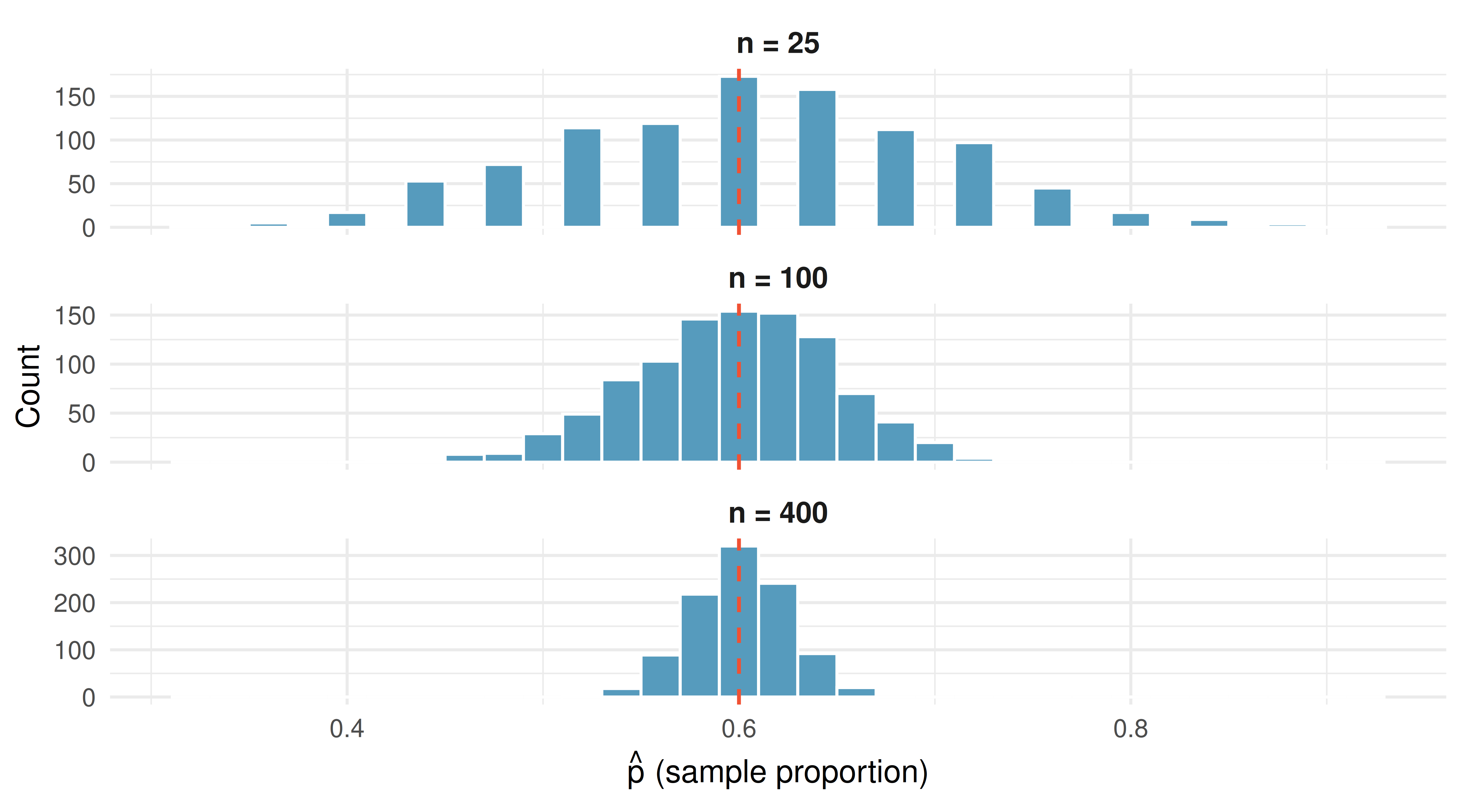
Figure 6.2 shows this dramatically: with \(n = 25\), individual sample proportions range from about 0.35 to 0.85. With \(n = 400\), they are tightly clustered between 0.55 and 0.65.

Predict → Do → Explain. The three properties above — center, spread, and shape — hold for any statistic. Open the Sampling Distribution Lab to build the sampling distribution of the sample mean from a right-skewed population. The gated activity opens with a Predict step (commit to the distribution’s shape, center, and how the spread changes as \(n\) grows before you draw), walks you through drawing at \(n = 5\) vs. \(n = 30\) with a reality-check gate at each stage, and closes with an Explain step where you articulate why the sampling distribution ends up centered at \(\mu\) and roughly bell-shaped even when the population is not. Two distinctions the lab is designed to make crisp: more samples fills in the same distribution, but larger \(n\) produces a different, narrower one. Your predictions and explanation save locally in the tool, so you can return to your work on the same device.

Self-check

At \(n = 5\) the sampling distribution is still somewhat right-skewed and fairly wide; by \(n = 30\) it is noticeably narrower and nearly symmetric — a first glimpse of the Central Limit Theorem: averages of independent draws become approximately normal as \(n\) grows, even when the population is not. The center stays put at the population mean because averaging is unbiased — no amount of skew shifts it. The spread shrinks because \(\sigma/\sqrt{n}\) shrinks: quadrupling \(n\) cuts the standard error roughly in half.

6.4 Standard error

We need a single number that quantifies how much a statistic varies from sample to sample. That number is the standard error.

The standard error (SE) of a statistic is the standard deviation of its sampling distribution. It measures the typical distance between a sample statistic and the population parameter.

A small standard error means the statistic tends to fall close to the parameter (precise estimate). A large standard error means the statistic could plausibly fall far from the parameter (imprecise estimate).

Do not confuse the standard error with the standard deviation of the data:

• The standard deviation (\(s\) or \(\sigma\)) measures how much individual observations vary around the mean.
• The standard error (SE) measures how much a sample statistic varies around the population parameter from sample to sample.

The standard error is always smaller than the standard deviation (for samples larger than \(n = 1\)) because averaging reduces variability.

Figure 6.3: Comparing the data distribution (top) with the sampling distribution of the mean (bottom). Both are centered near the same value, but the sampling distribution is much narrower — its spread is the standard error, not the standard deviation. ↗ Try this live — regenerate this side-by-side comparison and vary \(n\) to watch the sampling distribution narrow further.

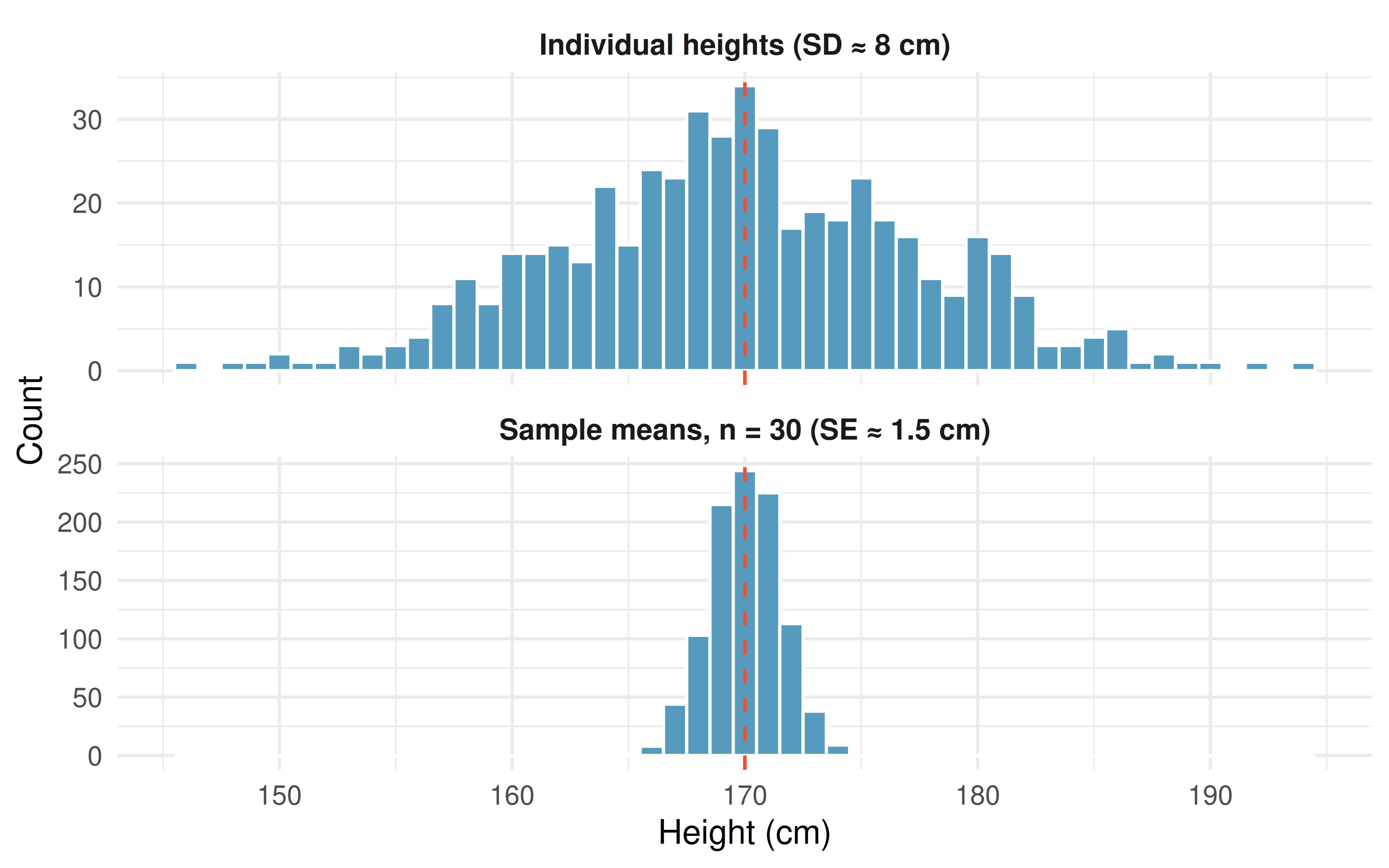
In Figure 6.3, the top panel shows how individual heights vary (SD \(\approx 8\) cm), while the bottom panel shows how sample means vary (SE \(\approx 1.5\) cm). Both are centered near \(\mu = 170\), but the sampling distribution of the mean is much narrower.

In the medical consultant example, \(\hat{p} = 3/62 = 0.048\). If we could take many samples of 62 patients from this consultant’s true patient population and compute \(\hat{p}\) each time, the standard deviation of all those \(\hat{p}\) values would be the standard error of \(\hat{p}\).

While we usually cannot literally take repeated samples, simulation methods (which we will explore in the randomization tests and bootstrap confidence intervals chapters) allow us to approximate the standard error. In this case, bootstrap simulations suggest that the standard error of \(\hat{p}\) is approximately 0.027. This means that if we could repeat the study many times, the sample complication rate would typically differ from the true complication rate by about 2.7 percentage points.

6.4.1 Why the standard error matters

The standard error is the engine of statistical inference. Here is why:

• Confidence intervals are built by going a certain number of standard errors above and below the point estimate. A rough 95% confidence interval is:

  \[\text{statistic} \pm 2 \times SE\]

• Hypothesis tests compare an observed statistic to what we would expect under the null hypothesis. The comparison is made in units of standard errors: “Is the observed result more than 2 standard errors from the null value?”

• Sample size planning uses the standard error to determine how many observations are needed to achieve a desired level of precision.

In the coming chapters, we will use simulation to estimate the standard error. In later chapters (Unit 3), we will use mathematical formulas to calculate it directly.

Two researchers both estimate the proportion of college students who prefer online textbooks. Researcher A surveys 100 students and finds \(\hat{p}_A = 0.62\) with \(SE_A = 0.049\). Researcher B surveys 400 students and finds \(\hat{p}_B = 0.58\) with \(SE_B = 0.025\).

1. Whose estimate is more precise? How do you know?
2. Why is Researcher B’s standard error smaller?

Show answer

1. Researcher B’s estimate is more precise because the standard error is smaller (0.025 < 0.049), meaning the sample statistic is expected to be closer to the true parameter. (b) Researcher B surveyed four times as many students, and increasing the sample size reduces the standard error.

6.5 Looking ahead

This chapter has established the core vocabulary and ideas that drive all of statistical inference:

• We want to know about parameters but can only observe statistics.
• Statistics vary from sample to sample — this is sampling variability.
• The pattern of this variation is described by the sampling distribution.
• The standard error quantifies the typical amount of sampling variability.

The fundamental question of inference is: Given the sampling variability we expect, is the pattern in our data real, or could it have happened by chance?

In the next three chapters, we will answer this question using three different approaches — all rooted in simulation:

• Randomization Tests: Shuffle the data to see what differences look like when there is no real effect. If the observed difference is extreme compared to the shuffled results, we have evidence of a real effect.
• Bootstrap Confidence Intervals: Resample from the data to approximate the sampling distribution, and use it to construct a range of plausible values for the parameter.
• Sampling Distributions via Simulation: Connect the simulation results from the randomization tests and bootstrap confidence intervals chapters to mathematical theory, setting the stage for the formula-based methods in Unit 3.

The goal of Unit 2 is to build your intuition for inference. The formulas will come later; the ideas come first.

6.6 Chapter review

6.6.1 Summary

• A population parameter is a fixed but unknown numerical summary of the population. A sample statistic (point estimate) is computed from data and serves as our best guess of the parameter.
• Different samples from the same population yield different statistics. This is sampling variability — it is not a mistake, but a fundamental feature of working with samples.
• The sampling distribution of a statistic describes how the statistic varies across all possible samples of a given size. It is typically centered at the parameter, and its spread decreases as sample size increases.
• The standard error is the standard deviation of the sampling distribution. It measures the precision of the statistic as an estimate of the parameter.
• The standard error is not the same as the standard deviation of the data. The standard deviation measures variability of individual observations; the standard error measures variability of a statistic.
• Larger samples produce smaller standard errors, meaning more precise estimates.

6.6.2 Key terms

Term	Definition
Population parameter	A fixed numerical summary of the entire population (e.g., \(p\), \(\mu\))
Sample statistic	A numerical summary computed from sample data (e.g., \(\hat{p}\), \(\bar{x}\))
Point estimate	Another name for sample statistic; our best guess at the parameter
Sampling variability	The fact that different samples produce different statistics
Sampling distribution	The distribution of a statistic over all possible samples of a given size
Standard error (SE)	The standard deviation of the sampling distribution

6.7 Exercises

Answers to odd-numbered exercises are provided in the Exercise Solutions appendix at the back of the book.

1. Identify the parameter, I. For each of the following situations, state whether the parameter of interest is a mean or a proportion. It may be helpful to examine whether individual responses are numerical or categorical.

1. In a survey, 100 college students are asked how many hours per week they spend on the Internet.

2. In a survey, 100 college students are asked: “What percentage of the time you spend on the Internet is part of your course work?”

3. In a survey, 100 college students are asked whether they cited information from Wikipedia in their papers.

4. In a survey, 100 college students are asked what percentage of their total weekly spending is on alcoholic beverages.

5. In a sample of 100 recent college graduates, it is found that 85 percent expect to get a job within one year of their graduation date.

2. Identify the parameter, II. For each of the following situations, state whether the parameter of interest is a mean or a proportion.

1. A poll shows that 64% of Americans personally worry a great deal about federal spending and the budget deficit.

2. A survey reports that local TV news has shown a 17% increase in revenue within a two year period while newspaper revenues decreased by 6.4% during this time period.

3. In a survey, high school and college students are asked whether they use geolocation services on their smart phones.

4. In a survey, smart phone users are asked whether they use a web-based taxi service.

5. In a survey, smart phone users are asked how many times they used a web-based taxi service over the last year.

3. Sample size and the sampling distribution. A researcher plans to estimate the mean sleep hours per night for full-time college students in the U.S. She considers three possible sample sizes: \(n = 25\), \(n = 100\), and \(n = 400\). In each case, she would draw a simple random sample and compute \(\bar{x}\); the sampling distribution describes how \(\bar{x}\) varies across all possible samples of that size.

1. As \(n\) grows from 25 to 400, what happens to the center of the sampling distribution? Why?

2. As \(n\) grows from 25 to 400, what happens to the spread (standard error) of the sampling distribution? Give a rough factor: quadrupling \(n\) from 25 to 100 changes the standard error by roughly what?

3. As \(n\) grows from 25 to 400, what happens to the shape of the sampling distribution (assuming the population is not extremely skewed)? Describe what you would expect to see if you drew the histogram at each sample size.

4. Which of the three sample sizes gives the most precise estimate of the population mean? Which requires the most resources to collect? Briefly discuss the trade-off.

Show answer

1. The center stays the same at the population mean \(\mu\). The sample mean is an unbiased estimator, so its long-run average equals \(\mu\) regardless of sample size. Bigger samples don’t shift the target, they hit it more precisely.

2. The spread decreases as \(n\) grows. The typical distance from the center — the standard error — shrinks. As a rule of thumb, quadrupling \(n\) from 25 to 100 cuts the standard error roughly in half; going from 25 to 400 cuts it to about a quarter.

3. The shape becomes more symmetric and bell-shaped. At \(n = 25\) the sampling distribution can still look a bit lumpy or skewed (depending on the population); by \(n = 400\) it usually looks like a smooth mound. You’ll see this pattern formalized in a later chapter.

4. \(n = 400\) gives the most precise estimate (smallest standard error) but requires the most data collection effort. \(n = 25\) is cheap but has 4× the standard error of \(n = 400\). The typical study picks the smallest \(n\) that meets the precision target the research question demands.

4. Statistic vs. parameter with correct notation. For each described study, identify the population parameter and the sample statistic. For each, state whether it is a mean or a proportion, and write it with the correct symbol.

1. A national poll of 800 US adults finds that 42% support a proposed carbon tax. The pollster wants to estimate the true percentage of all US adults who support the tax.

2. A researcher measures the resting heart rate of 60 randomly-selected adult women in a city and finds a sample mean of 71 beats per minute. She wants to estimate the mean resting heart rate for the population of all adult women in the city.

3. A company tests 200 randomly-selected components off the assembly line and finds 5 defective. The quality engineer wants to estimate the long-run defect rate on this line.

4. In each of (a)–(c), which of the two — parameter or statistic — is known exactly, and which is being estimated?

Show answer

1. Parameter: the proportion of all US adults who support the tax, written \(p\) (unknown). Statistic: the sample proportion \(\hat{p} = 0.42\) (a proportion).

2. Parameter: the mean resting heart rate of all adult women in the city, written \(\mu\) (unknown). Statistic: the sample mean \(\bar{x} = 71\) (a mean).

3. Parameter: the true defect proportion \(p\) on this line (unknown). Statistic: the sample proportion \(\hat{p} = 5/200 = 0.025\) (a proportion).

4. In every case the statistic is known exactly (we computed it from the sample); the parameter is what we’re estimating. That’s the whole point of statistical inference: use what we can see (statistic) to draw conclusions about what we can’t (parameter).

5. Data distribution or sampling distribution? For each of the following descriptions, decide whether the histogram would show a data distribution (the distribution of individual observations) or a sampling distribution (the distribution of a sample statistic across many samples). Justify each in one sentence.

1. A histogram of the ages of all 1,200 patients admitted to a hospital ward last year.

2. A histogram of the mean age from each of 500 random samples of 30 patients drawn from those 1,200.

3. A dotplot showing the proportion of red beads for each of 400 people, where each person independently scooped a sample of 50 beads from the same bowl.

4. A histogram of the SAT scores from a random sample of 250 high-school seniors.

5. Which of the four would typically be narrower — a data distribution or a sampling distribution built from the same population? Explain in one sentence.

Show answer

1. Data distribution. Each observation is one patient’s age; no averaging or summarizing across samples.

2. Sampling distribution. Each observation is the mean of a sample of 30 patients — a statistic, not an individual value.

3. Sampling distribution. Each observation is a sample proportion \(\hat{p}\) from one person’s sample; the collection of 400 \(\hat{p}\) values is the sampling distribution.

4. Data distribution. Each observation is one student’s SAT score; no summarizing across samples.

5. The sampling distribution is narrower. Averaging (or otherwise summarizing) many observations dampens out extremes — the SE of \(\bar{x}\) is \(\sigma/\sqrt{n}\), which is always smaller than \(\sigma\) once \(n > 1\).

6. Reading a sampling distribution. The histogram below was built by drawing 1,000 random samples of size \(n = 40\) from a large population and recording the sample proportion \(\hat{p}\) (the proportion of “yes” responses to a survey question) for each. The true population proportion is \(p = 0.50\).

Figure 6.4: 1,000 sample proportions \(\hat{p}\) from samples of size \(n = 40\), drawn from a population with \(p = 0.50\).

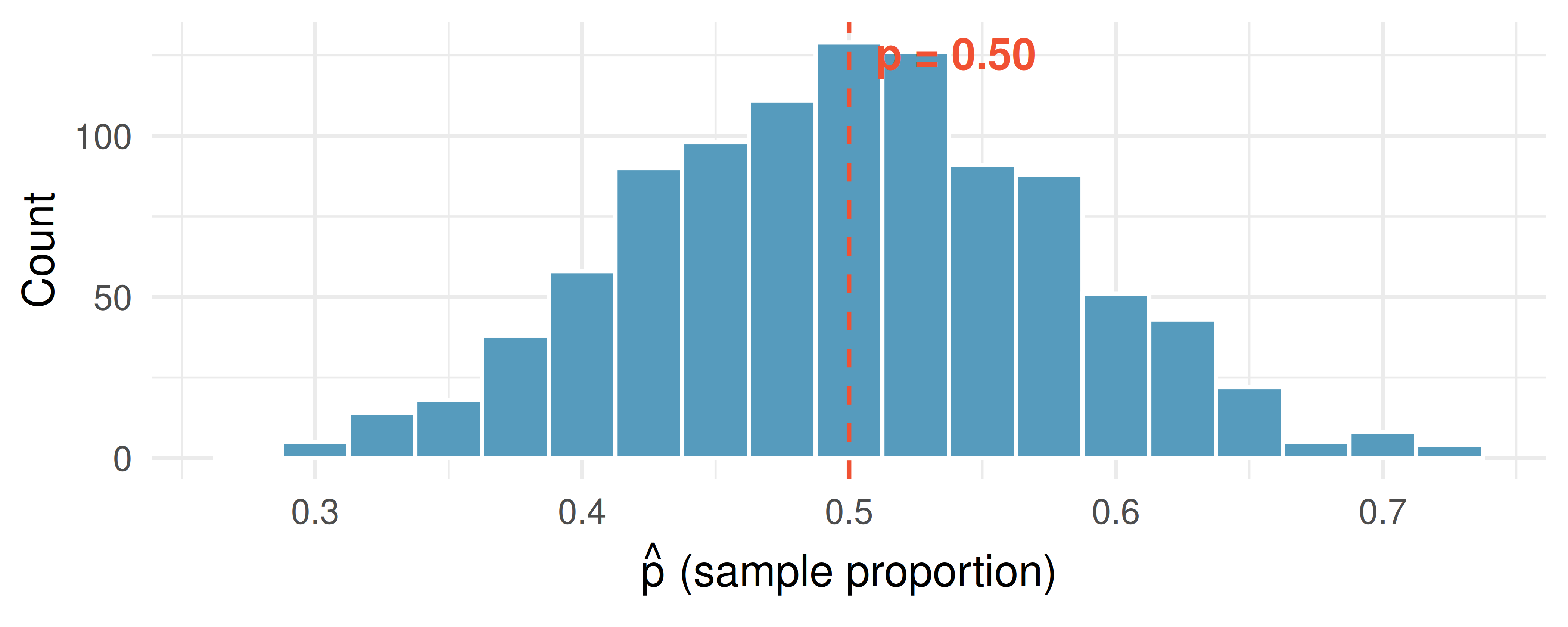
1. Where is the sampling distribution centered? How does that compare to the true \(p\)?

2. Describe the shape of the sampling distribution.

3. Estimate the standard error of \(\hat{p}\) by eyeballing the picture. (Recall: the SE is the standard deviation of the sampling distribution — roughly, the typical distance from the center.)

4. Suppose the samples were instead of size \(n = 160\) (four times as large). Describe how the picture would change. In particular, roughly what would the new standard error be?

Show answer

1. Centered at \(\hat{p} \approx 0.50\), matching the true parameter \(p = 0.50\). This is what “the sampling distribution is centered at the parameter” means in practice.

2. Approximately symmetric and bell-shaped — a common feature of sampling distributions when the sample size is large enough.

3. Most values fall within about \(\pm 0.08\) of the center, so the standard error is roughly 0.08 (or approximately \(\sqrt{0.5 \cdot 0.5 / 40} = 0.079\), which matches).

4. Quadrupling \(n\) from 40 to 160 cuts the standard error roughly in half: SE would drop from about 0.08 to about 0.04. The picture would still be centered at 0.50 and still bell-shaped, but noticeably narrower — most \(\hat{p}\) values would now fall within about \(\pm 0.04\) of the center.

↗ Try this yourself — the Sampling Distribution Lab lets you regenerate this picture live and drag the sliders to see what happens at other \(n\) or \(p\).

7. Standard deviation vs. standard error. A study of 400 college students reports sample mean sleep \(\bar{x} = 6.8\) hours per night, sample standard deviation \(s = 1.4\) hours, and standard error of the mean \(\text{SE}(\bar{x}) = 0.07\) hours. For each of the following statements, decide whether \(s\) or \(\text{SE}(\bar{x})\) is the appropriate number, and explain briefly.

1. “In this sample, a typical student’s sleep is within a few hours of 6.8.”

2. “If we drew a fresh sample of 400 college students and recomputed the mean, the new \(\bar{x}\) would typically be within a tenth of an hour of the true population mean.”

3. A researcher writes: “The variability in sleep hours across students in this sample is about 1.4 hours.” Is she describing \(s\) or \(\text{SE}(\bar{x})\)?

4. Explain why \(\text{SE}(\bar{x})\) is so much smaller than \(s\) for this study.

Show answer

1. \(s = 1.4\) hours. “A typical student” is about individual variation — that’s the sample standard deviation. \(s\) says most students sleep within roughly 1.4 hours of 6.8.

2. \(\text{SE}(\bar{x}) = 0.07\) hours. “How much would the sample mean \(\bar{x}\) vary from sample to sample” is exactly the standard error. Fresh samples of 400 would give \(\bar{x}\) values typically within about 0.07 of the population mean.

3. \(s\). She’s describing variability across students — that’s the standard deviation of the data.

4. Averaging 400 observations damps out individual variability. The formula \(\text{SE}(\bar{x}) = s/\sqrt{n} = 1.4 / \sqrt{400} = 1.4/20 = 0.07\) makes it explicit: dividing by \(\sqrt{n} = 20\) shrinks the spread by a factor of 20 relative to \(s\).

8. What a reported standard error tells you. A national polling firm surveys 1,067 US adults and reports that 51% support a particular ballot measure, with a margin of error of \(\pm 3\) percentage points at 95% confidence (which corresponds roughly to \(2 \cdot \text{SE} \approx 0.03\), i.e., \(\text{SE} \approx 0.015\)).

1. If the firm’s polling procedure were repeated many times with fresh random samples of 1,067 adults, roughly what would a picture of all their \(\hat{p}\) values look like? Describe the center and spread.

2. Would you be surprised if a different firm, using the same methodology and a fresh sample of 1,067 adults, reported 48% support? What about 40% support? Explain each briefly using the SE.

3. Suppose the firm doubled its sample size to about 2,134 adults. Roughly what would the new SE and margin of error become? (Hint: SE scales like \(1/\sqrt{n}\), so doubling \(n\) multiplies SE by \(1/\sqrt{2} \approx 0.71\).)

4. A political commentator sees the poll and writes: “Support is definitely between 48% and 54%.” What’s wrong with the word definitely?

Show answer

1. Roughly a bell curve centered at the true population support proportion, with a standard deviation of about 0.015 (1.5 percentage points). Most repeated polls would land within about \(\pm 0.03\) of the true \(p\).

2. 48% would not be surprising — that’s within 1 SE (0.015) of 51%, well inside typical sampling variability. 40% would be very surprising — that’s about 7 SEs away from 51%, which almost never happens by sampling variability alone; it would suggest a real difference in the population or a methodology problem.

3. New SE \(\approx 0.015 \times 0.71 \approx 0.011\), so the margin of error would drop from \(\pm 3\) to about \(\pm 2.1\) percentage points. Doubling \(n\) gives modest precision gain, not double.

4. The interval is a statistical range, not a certain one. It’s built to trap the true \(p\) about 95% of the time across repeated polls — not to guarantee \(p\) is inside for this specific poll. “Definitely” overstates what a CI can promise.

9. Match the sampling distributions. Below are four histograms, each built by drawing 1,000 random samples and recording the sample proportion \(\hat{p}\) each time. They come from four different \((n, p)\) combinations:

• \((n = 25, \, p = 0.20)\)
• \((n = 100, \, p = 0.20)\)
• \((n = 25, \, p = 0.50)\)
• \((n = 100, \, p = 0.50)\)

Match each panel (A, B, C, D) to its combination, using only what you can see. Then briefly justify each match in one sentence: what feature of the picture told you center (relates to \(p\)) versus spread (relates to \(n\))?

Figure 6.5: Four sampling distributions of \(\hat{p}\). Each built from 1,000 random samples.

Show answer

• A: \((n = 100, \, p = 0.20)\) — centered near 0.20, narrow spread.
• B: \((n = 25, \, p = 0.50)\) — centered near 0.50, wide spread.
• C: \((n = 25, \, p = 0.20)\) — centered near 0.20, wide spread.
• D: \((n = 100, \, p = 0.50)\) — centered near 0.50, narrow spread.

The center told you \(p\): whichever bar-mass mode sits near 0.20 vs. 0.50. The spread told you \(n\): the wider histograms (twice the visible width) are \(n = 25\); the tighter ones are \(n = 100\). Quadrupling \(n\) (25 → 100) roughly halves the spread — you can see it directly.

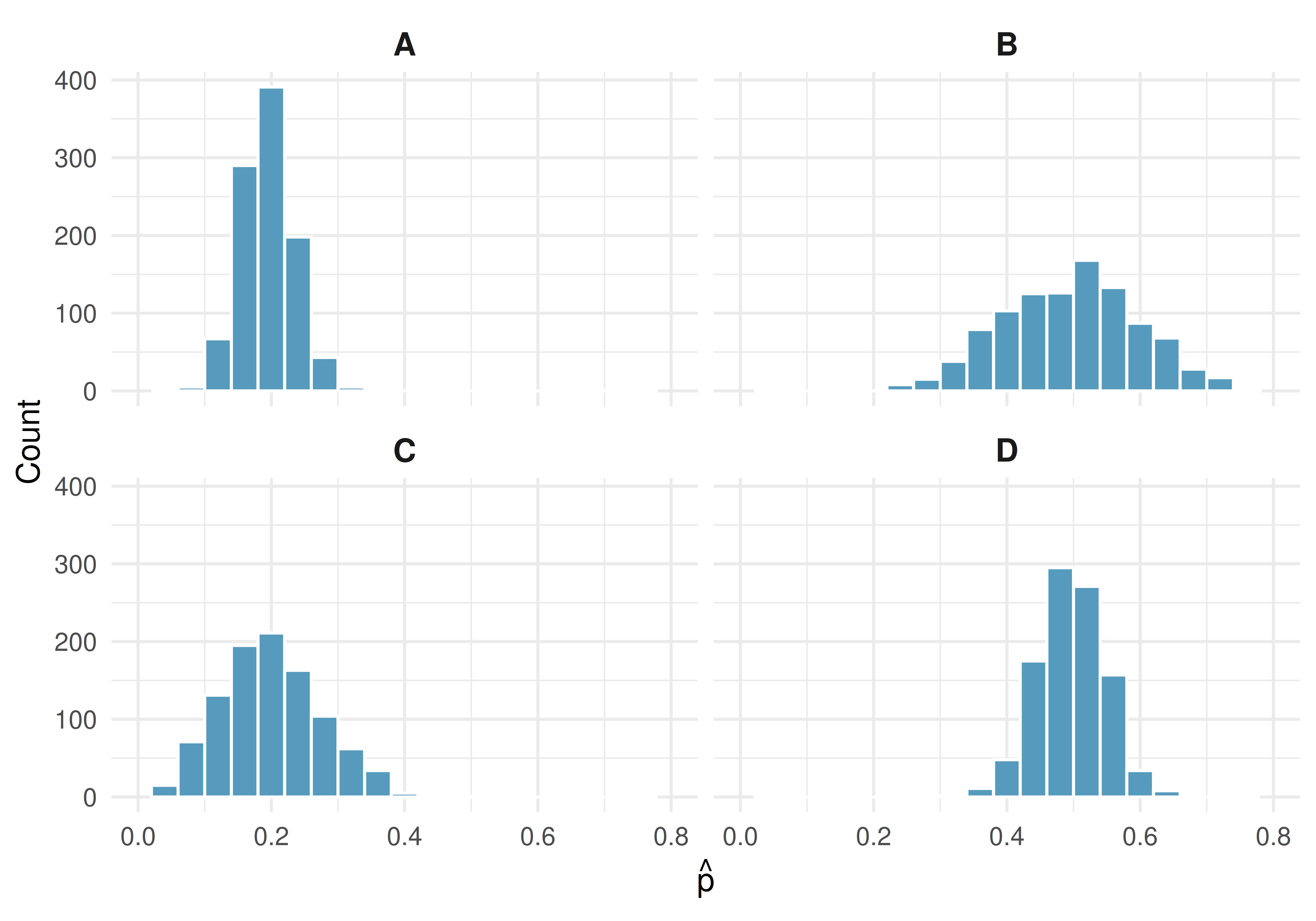
↗ Try this yourself — in the Sampling Distribution Lab, drive the \(n\) and \(p\) sliders to any of the four combos and watch the histogram redraw. Does it match the panel you assigned it to?

10. Estimate the standard error from a dot plot. The dot plot below shows the sample means \(\bar{x}\) from 50 random samples of 30 college students each. In each sample, the researcher measured hours of sleep per night; the population mean is \(\mu = 7.0\) hours.

Figure 6.6: 50 sample means \(\bar{x}\) from repeated samples of size \(n = 30\). Population mean \(\mu = 7.0\) hours.

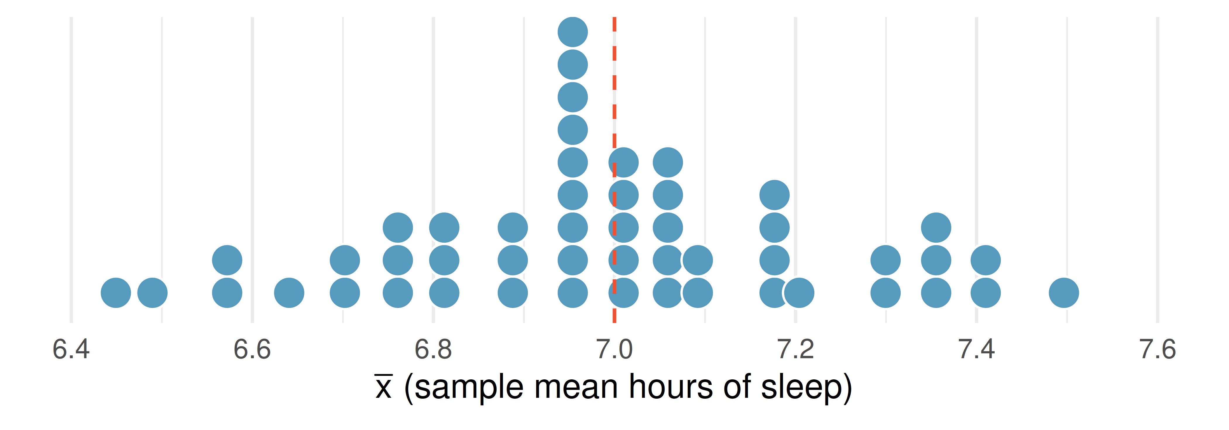
1. Where is the sampling distribution of \(\bar{x}\) centered? How does that compare to the population mean \(\mu = 7.0\)?

2. Recall: the standard error of \(\bar{x}\) is the standard deviation of the sampling distribution — roughly, the typical distance of a dot from the center. Estimate the SE from the picture. (A rough eyeball: the range from lowest to highest dot spans about \(\pm 2\) SE if the shape is roughly bell-shaped.)

3. A student computes the standard error using the population SD \(\sigma = 1.4\) hours: \(\sigma / \sqrt{n} = 1.4 / \sqrt{30} \approx 0.26\). How does that compare to your visual estimate in (b)?

4. If the researcher had drawn samples of size \(n = 120\) instead of \(n = 30\), how would the width of this dot plot change? Give a rough factor.

Show answer

1. Centered at about \(\bar{x} = 7.0\), matching the population mean \(\mu\). The sample mean is unbiased — averaging many \(\bar{x}\)’s recovers \(\mu\).

2. Dots span roughly 6.5 to 7.5, so the total spread is about 1.0 hour. That’s roughly \(4 \cdot \text{SE}\), giving SE ≈ 0.25 hours. (Or: most dots fall within about \(\pm 0.25\) of 7.0, which directly reads as the SE.)

3. Very close — \(\sigma / \sqrt{n} \approx 0.26\) matches the visual estimate of about 0.25. The picture is a direct visual read of the same number the formula gives.

4. Quadrupling \(n\) from 30 to 120 cuts the SE in half: SE would drop from about 0.26 to about 0.13. The dot plot would look about half as wide — most dots would fall between roughly 6.87 and 7.13.

↗ Try this yourself — the Sampling Distribution Lab lets you regenerate a dot plot with these settings, then drive \(n\) up to 120 and watch the spread shrink.

StatLens Exercises

These exercises focus on the ideas behind sampling variability: telling a parameter from a statistic, a sampling distribution from a data distribution, and reading the standard error. Where a link is given, let StatLens do the simulating and spend your effort on the reasoning.

1. Parameter or statistic? A university has 14,000 undergraduates. A researcher surveys a random sample of 200 of them and finds that 132 work at least 10 hours a week.

   1. Identify the population and the sample.
   2. Is the value \(132/200 = 0.66\) a parameter or a statistic? Give its symbol.
   3. Is the true fraction of all 14,000 undergraduates who work 10+ hours a parameter or a statistic? Give its symbol. Is its value known?

2. Sampling distribution vs. data distribution. A nurse records the resting heart rate of every patient in a large clinic, then also computes the mean heart rate of each day’s batch of 40 patients over many days.

   1. Which collection of numbers forms a data distribution — the individual heart rates, or the daily means?
   2. Which forms a sampling distribution?
   3. Which of the two distributions has the larger spread, and why?

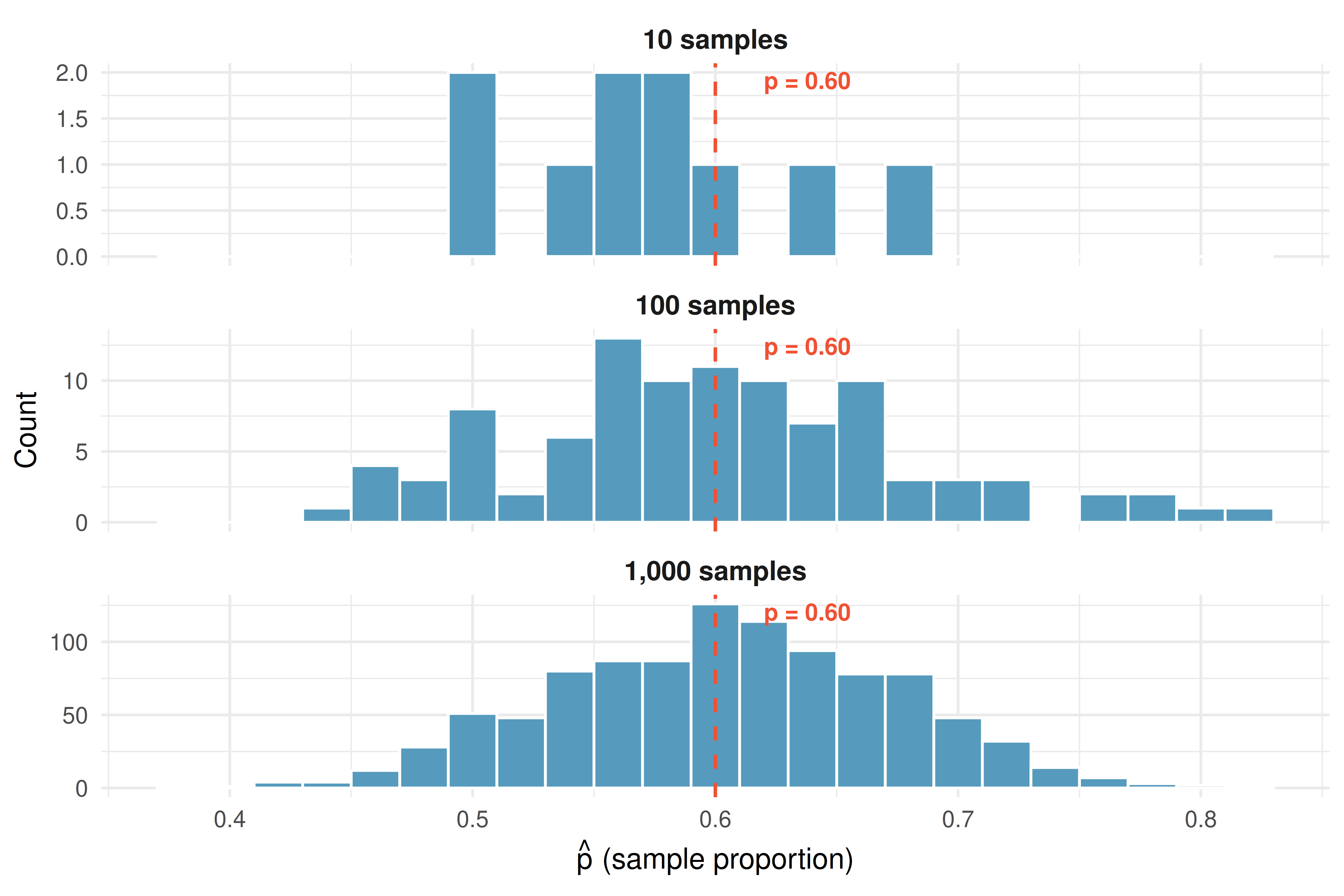
3. Predict, then check: two different knobs. You saw the effect of sample size on the sampling distribution in the three-panel figure earlier in this chapter (all three centered at \(p = 0.60\), spread shrinking as \(n\) grew). Now drive it yourself: first, write your predictions; then open the Sampling Distribution Simulator and choose the right-skewed population.

   1. Predict the shape of the sampling distribution of \(\bar{x}\) for \(n = 5\) (as skewed as the population, less skewed, or symmetric?). Then set \(n = 5\), draw many samples, and compare to your prediction.
   2. With \(n = 5\) still set, draw even more samples. Does the spread shrink, or does the distribution just fill in? Now switch to \(n = 50\). Which of the two actions — more samples or larger \(n\) — changed the spread?
   3. The tool shows the theoretical standard error \(\sigma/\sqrt{n}\) and the observed SD of the sample means. Why should these two numbers be close?

4. Interpret the standard error. A polling firm estimates support for a ballot measure from a random sample and reports \(\hat{p} = 0.47\) with a standard error of \(0.02\).

   1. In plain language, what does the standard error of \(0.02\) tell you?
   2. Roughly how far from the true proportion might \(\hat{p}\) reasonably be? (Use the “\(\pm 2\,SE\)” idea.)
   3. The firm wants to halve the standard error for its next poll. By what factor must it increase the sample size, and why?

5. Spot the mistake. A student writes: “I took one sample of 60 students and got \(\bar{x} = 7.1\) hours of sleep. The standard error was 0.3, so 95% of students sleep between about 6.5 and 7.7 hours.”

   1. What has the student confused?
   2. What does the interval \(7.1 \pm 2(0.3)\) actually describe?