Project: Association Between Two Categorical Variables

Project — Chi-Square Test of Independence. Carry out the analysis in Jamovi (or R) and communicate the result. The graded skills are framing the association question, checking the expected-count condition, and interpreting the test in context.

The question

Few airplane debates are as heated as whether it’s acceptable to recline your seat. FiveThirtyEight ran a national survey on flying etiquette, asking travelers whether reclining is rude — and recording each respondent’s age.

Is a flyer’s opinion on reclining associated with their age?

The data

flying_etiquette.csv holds the survey responses (about 1,040 people; ~843 answered both questions here). You’ll use two categorical variables: recline_rude (No, Somewhat, Very — how rude is it to recline?) and age (18-29, 30-44, 45-60, > 60). Source: FiveThirtyEight, “Hey, You Should Stop Reclining Your Airplane Seat.”

Plan it first

1. Variables. Confirm both variables are categorical and give the size of the table (rows × columns).
2. Hypotheses. State \(H_0\) and \(H_A\) for a test of independence in words (opinion on reclining and age are independent vs. associated).
3. Eyeball it. Look at the row percentages (the opinion mix within each age group). Can you tell for sure whether opinion depends on age, or could the differences be chance? This is the judgment the test makes rigorous.
4. Procedure & condition. Two categorical variables, “are they associated?” → chi-square test of independence. It needs expected counts that aren’t too small (a common rule: each ≥ 5) — what will you check?

Do the analysis

Jamovi

1. Open flying_etiquette.csv.
2. Frequencies → Independent Samples (χ² test of association). Rows: age; Columns: recline_rude.
3. Request the χ² test, expected counts, and row percentages.
4. Read off the table, confirm expected counts are large enough, and record χ² and the p-value.

(Jamovi screenshots to be added.)

R

library(infer)
library(dplyr)
library(readr)
library(ggplot2)

flying <- read_csv("../datasets/flying_etiquette.csv")

# Keep respondents who answered both questions; order the categories
fly <- flying |>
  filter(!is.na(recline_rude), !is.na(age)) |>
  mutate(age          = factor(age, levels = c("18-29", "30-44", "45-60", "> 60")),
         recline_rude = factor(recline_rude, levels = c("No", "Somewhat", "Very")))

# Contingency table
tab <- table(fly$age, fly$recline_rude)
tab

       
         No Somewhat Very
  18-29  78       74   20
  30-44 143       64   15
  45-60 140       80   14
  > 60  133       61   21

# Row percentages: the opinion mix within each age group (try to eyeball it)
round(100 * prop.table(tab, 1), 0)

       
        No Somewhat Very
  18-29 45       43   12
  30-44 64       29    7
  45-60 60       34    6
  > 60  62       28   10

# Chi-square test of independence (infer)
fly |> chisq_test(recline_rude ~ age)

# A tibble: 1 × 3
  statistic chisq_df p_value
      <dbl>    <int>   <dbl>
1      19.8        6 0.00305

# Condition check: smallest expected count (rule of thumb: each >= 5)
cat("Smallest expected count:", round(min(chisq.test(tab)$expected), 1), "\n")

Smallest expected count: 14.3 

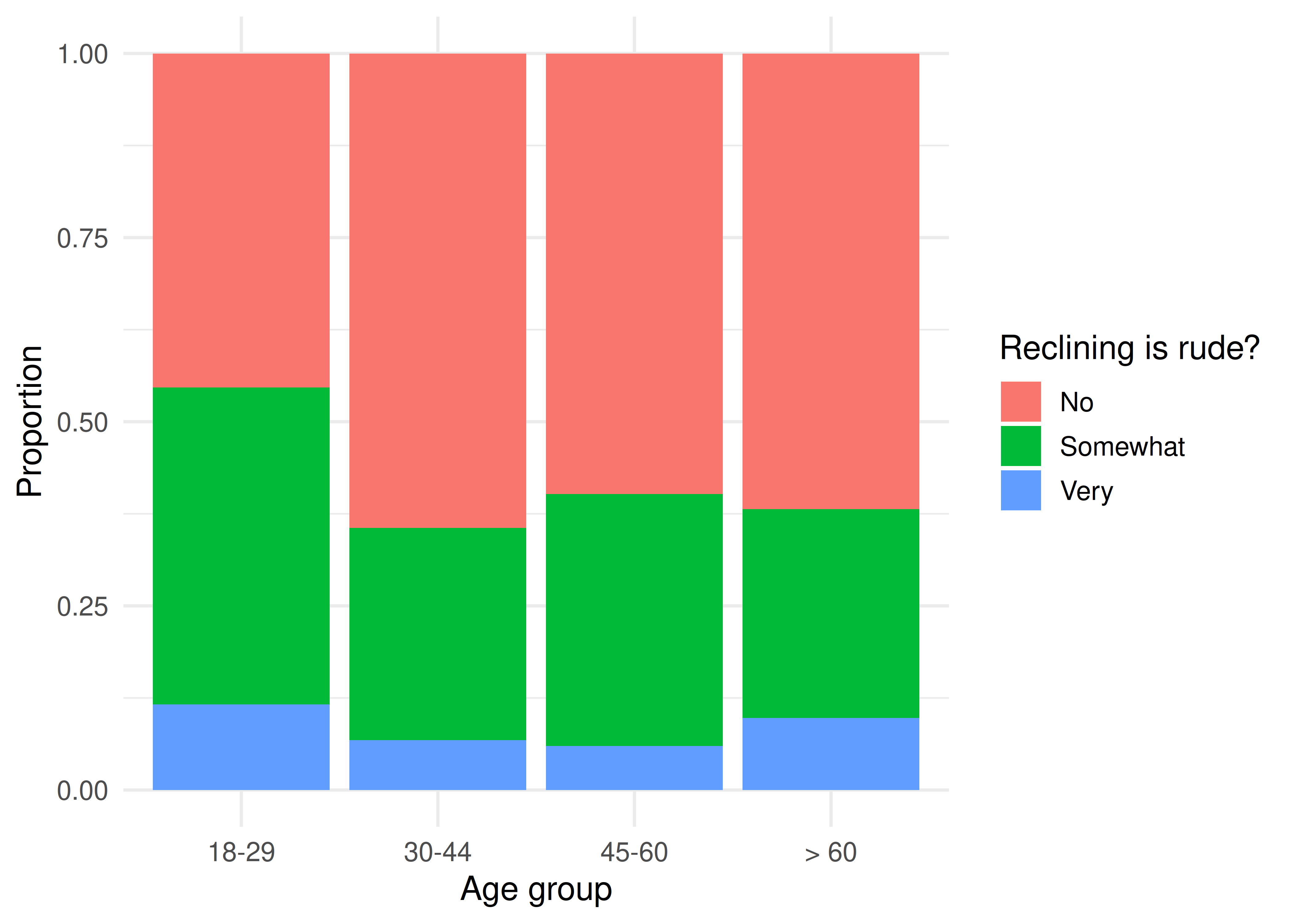
ggplot(fly, aes(age, fill = recline_rude)) +
  geom_bar(position = "fill") +
  labs(x = "Age group", y = "Proportion", fill = "Reclining is rude?") +
  theme_minimal(base_size = 13)

Opinion on reclining by age group. Younger flyers are the most likely to call reclining rude — but is the difference real or noise?

Your deliverable

Submit a short report containing all of:

1. Graphic — a labeled stacked (or side-by-side) bar chart showing the opinion mix by age group.
2. Numerical result — the contingency table, the χ² statistic, the degrees of freedom, and the p-value.
3. Conditions — one sentence confirming the expected counts are large enough for the chi-square approximation.
4. Conclusion in context — 3–4 sentences: is there discernible evidence that opinion on reclining is associated with age? Describe the pattern (who finds it rudest?), note how the test settled what the percentages alone left uncertain, and stress that association is not causation.
5. One limitation — e.g., this is a single online survey; opinions may shift over time or differ by who chose to respond.

How it’s graded

Criterion	What we look for
Appropriate, labeled graphic	opinion mix by group, axes/legend labeled
Procedure & conditions	chi-square independence identified; expected counts checked
Correct numerical result	table, χ², df, p-value reported correctly
Conclusion in context	discernibility + the age pattern + association ≠ causation
Communication	clear, correct interpretation

Warm up first. Explore expected counts and the χ² statistic in the Chi-Square tool before writing your report.