26 Expected Value and Variance
How much revenue should a bookstore expect per student? How much variability should a stock investor anticipate in their portfolio? These questions require us to summarize a random variable’s distribution with just two numbers: its expected value (center) and variance (spread). In this chapter, we define these quantities, develop useful computational properties, and extend them to linear combinations of random variables. These tools will be essential when we study the binomial and normal distributions in the chapters that follow.
26.1 Expected value of a random variable
We introduced random variables in the random variables chapter. Now we develop the tools to summarize them numerically, starting with the expected value — the long-run average of a random variable.
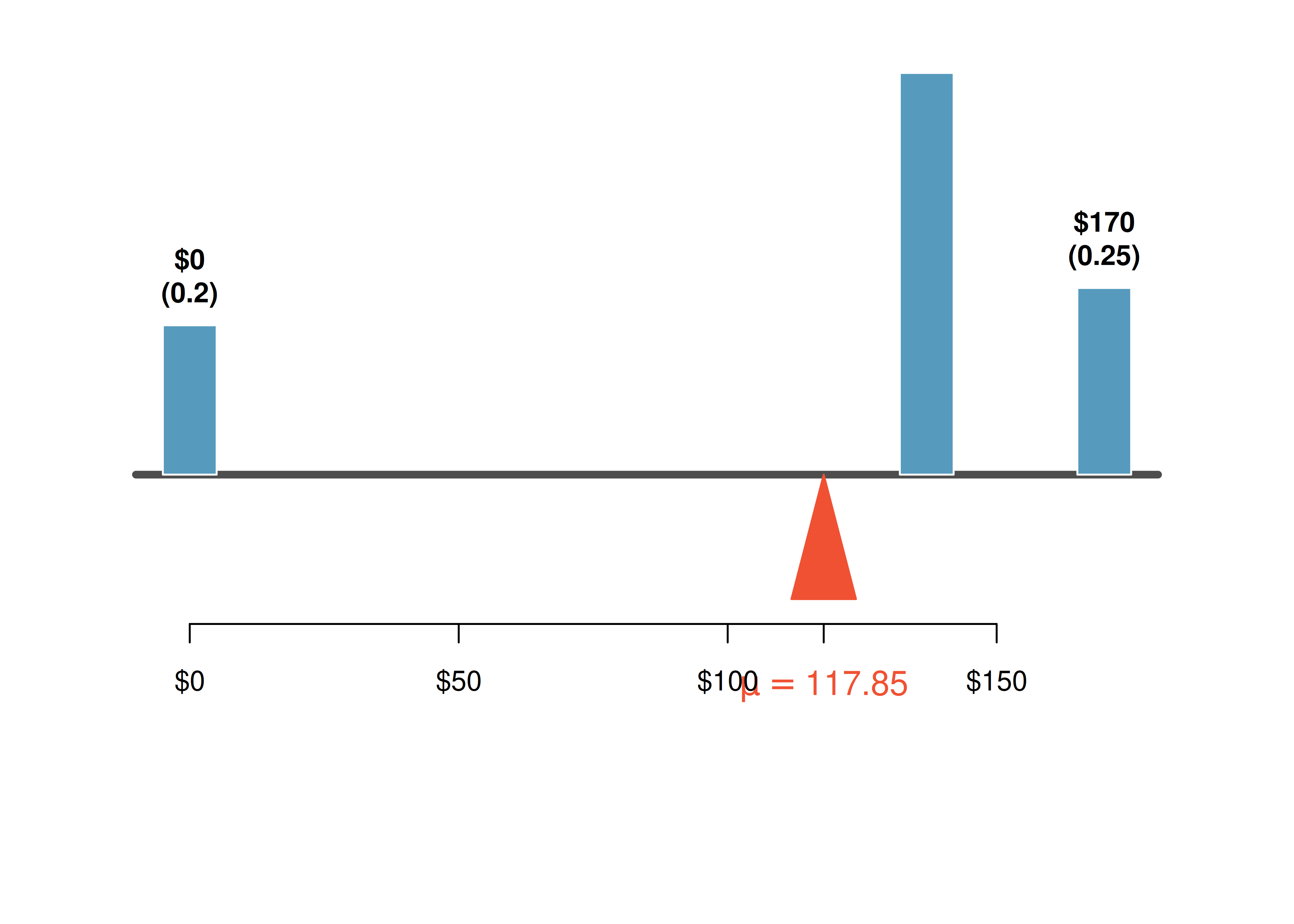
Two books are assigned for a statistics class: a textbook ($137) and a study guide ($33). From past experience, the bookstore knows that 20% of enrolled students buy neither book, 55% buy the textbook only, and 25% buy both books. If there are 100 students enrolled, how many books should the bookstore expect to sell?
About 20 students buy 0 books, 55 buy 1 book (55 books total), and 25 buy 2 books (50 books total). The bookstore should expect to sell about \(0 + 55 + 50 = 105\) books.
What is the average revenue per student?
The expected total revenue is \(\$0 \times 20 + \$137 \times 55 + \$170 \times 25 = \$11{,}785\), and there are 100 students. The expected revenue per student is \(\$11{,}785 / 100 = \$117.85\).
Notice that the “average revenue per student” was computed by multiplying each outcome by its probability and summing:
\[0 \times 0.20 + 137 \times 0.55 + 170 \times 0.25 = 117.85\]
This is the expected value of the random variable \(X\).
Expected value of a discrete random variable. If \(X\) takes outcomes \(x_1, x_2, \ldots, x_k\) with probabilities \(P(X = x_1), P(X = x_2), \ldots, P(X = x_k)\), the expected value of \(X\) is:
\[E(X) = x_1 \cdot P(X = x_1) + x_2 \cdot P(X = x_2) + \cdots + x_k \cdot P(X = x_k) = \sum_{i=1}^{k} x_i \, P(X = x_i)\]
The Greek letter \(\mu\) may be used in place of \(E(X)\).
The expected value represents the long-run average of the random variable. If we were to observe the random process many, many times, the average of all observed values would converge to \(E(X)\).
26.1.1 The expected value as a center of gravity
In physics, the expected value corresponds to the center of gravity (or balance point) of a distribution. Imagine cutting out the shape of a probability distribution from a piece of cardboard. The expected value is the point where you could balance the cutout on the tip of your finger. This is why we sometimes call \(E(X)\) the “mean” — it is exactly analogous to the sample mean \(\bar{x}\), but for a probability distribution rather than a data set.
A campus shuttle arrives every 10 minutes. The number of students boarding follows this distribution:
| \(x\) | 0 | 1 | 2 | 3 | 4 |
|---|---|---|---|---|---|
| \(P(X = x)\) | 0.10 | 0.25 | 0.35 | 0.20 | 0.10 |
What is the expected number of students who board?
Show answer
\(E(X) = 0(0.10) + 1(0.25) + 2(0.35) + 3(0.20) + 4(0.10) = 0 + 0.25 + 0.70 + 0.60 + 0.40 = 1.95\). On average, about 1.95 students board the shuttle at this stop.The expected value does not have to be a value that the random variable can actually take. In the shuttle example, \(E(X) = 1.95\), but you can never have 1.95 students board. The expected value is a long-run average, not a prediction of any single outcome.
26.2 Variance of a random variable
The expected value tells us where the center of a distribution lies, but it says nothing about the spread. The bookstore might want to know not just the average revenue per student, but how much that revenue varies from student to student.
Variance of a discrete random variable. If \(X\) takes outcomes \(x_1, \ldots, x_k\) with probabilities \(P(X = x_1), \ldots, P(X = x_k)\) and expected value \(\mu = E(X)\), then the variance of \(X\) is:
\[\text{Var}(X) = \sigma^2 = \sum_{i=1}^{k} (x_i - \mu)^2 \, P(X = x_i)\]
The standard deviation is \(\sigma = \sqrt{\text{Var}(X)}\).
The variance is the average squared deviation from the mean, weighted by the probabilities. The standard deviation has the same units as \(X\), which makes it more interpretable.
Compute the variance and standard deviation of the bookstore revenue per student.
We organize the calculation in a table with \(\mu = 117.85\):
| \(x_1 = 0\) | \(x_2 = 137\) | \(x_3 = 170\) | Total | |
|---|---|---|---|---|
| \(P(X = x_i)\) | 0.20 | 0.55 | 0.25 | |
| \(x_i - \mu\) | \(-117.85\) | \(19.15\) | \(52.15\) | |
| \((x_i - \mu)^2\) | \(13{,}888.6\) | \(366.7\) | \(2{,}719.6\) | |
| \((x_i - \mu)^2 \cdot P(X = x_i)\) | \(2{,}777.7\) | \(201.7\) | \(679.9\) | \(3{,}659.3\) |
The variance is \(\sigma^2 = 3{,}659.3\) and the standard deviation is \(\sigma = \sqrt{3{,}659.3} = \$60.49\).
The bookstore also sells a chemistry textbook ($159) and supplement ($41). From past experience, 15% of chemistry students buy neither, 25% buy the textbook only, and 60% buy both. Let \(Y\) be the revenue from a single chemistry student. (a) Write out the probability distribution of \(Y\). (b) Compute \(E(Y)\). (c) Compute \(\text{SD}(Y)\).
Show answer
- \(Y\) takes values $0, $159, $200 with probabilities 0.15, 0.25, 0.60. (b) \(E(Y) = 0(0.15) + 159(0.25) + 200(0.60) = 0 + 39.75 + 120 = \$159.75\). (c) \(\text{Var}(Y) = (0 - 159.75)^2(0.15) + (159 - 159.75)^2(0.25) + (200 - 159.75)^2(0.60) = 3828.0 + 0.1 + 972.0 = 4800.1\), so \(\text{SD}(Y) = \sqrt{4800.1} \approx \$69.28\).
26.3 Properties of expected value
The expected value has several important algebraic properties that make it easy to work with. These properties follow from the definition but are worth stating explicitly because we will use them frequently.
Properties of expected value. For a random variable \(X\) and constants \(a\) and \(b\):
- Adding a constant shifts the mean: \(E(X + b) = E(X) + b\)
- Multiplying by a constant scales the mean: \(E(aX) = a \cdot E(X)\)
- General linear transformation: \(E(aX + b) = a \cdot E(X) + b\)
Why these make sense: If every student’s textbook cost increases by $10 (adding a constant \(b = 10\)), then the average cost also increases by $10. If the bookstore marks up all prices by 20% (multiplying by \(a = 1.20\)), then the average revenue also increases by 20%.
Suppose the bookstore offers a 10% discount on every book purchase. The discounted price is \(0.90 \times X\), where \(X\) is the original price. What is the expected revenue per student under the discount?
Using the property \(E(aX) = aE(X)\):
\[E(0.90X) = 0.90 \times E(X) = 0.90 \times 117.85 = \$106.07\]
The expected revenue per student drops from $117.85 to $106.07.
The bookstore charges a flat $5 processing fee in addition to book costs. If \(X\) is the cost of books and the total charge is \(Y = X + 5\), what is \(E(Y)\)?
Show answer
\(E(Y) = E(X + 5) = E(X) + 5 = 117.85 + 5 = \$122.85\).26.4 Properties of variance
Variance has different algebraic properties than expected value. The most important distinction: adding a constant does not change the variance.
Properties of variance. For a random variable \(X\) and constants \(a\) and \(b\):
- Adding a constant does not change variance: \(\text{Var}(X + b) = \text{Var}(X)\)
- Multiplying by a constant scales variance by the square: \(\text{Var}(aX) = a^2 \cdot \text{Var}(X)\)
- General linear transformation: \(\text{Var}(aX + b) = a^2 \cdot \text{Var}(X)\)
For standard deviations:
\[\text{SD}(aX + b) = |a| \cdot \text{SD}(X)\]
Why adding a constant does not change variance: If every student pays $5 more, the spread of payments does not change — everyone’s payment shifts by the same amount. The center moves, but the variability stays the same.
Why multiplying scales by the square: If every price is doubled (\(a = 2\)), then deviations from the mean are also doubled, so squared deviations are multiplied by \(2^2 = 4\).
For the bookstore revenue with \(\text{Var}(X) = 3{,}659.3\) and \(\sigma_X = \$60.49\):
- If a $5 fee is added: \(\text{Var}(X + 5) = \text{Var}(X) = 3{,}659.3\) and \(\text{SD}(X+5) = \$60.49\).
- If a 10% discount is applied: \(\text{Var}(0.90X) = 0.90^2 \times 3{,}659.3 = 0.81 \times 3{,}659.3 = 2{,}964.0\) and \(\text{SD}(0.90X) = 0.90 \times 60.49 = \$54.44\).
Suppose temperatures in Celsius are converted to Fahrenheit using \(F = 1.8C + 32\). If the standard deviation of daily high temperatures is \(\sigma_C = 5^\circ\text{C}\), what is the standard deviation in Fahrenheit?
Show answer
\(\text{SD}(1.8C + 32) = 1.8 \times \text{SD}(C) = 1.8 \times 5 = 9^\circ\text{F}\). The additive constant 32 does not affect the spread.26.5 Linear combinations of random variables
Sometimes the total outcome is best described as a sum of several random variables. For instance, a person’s total weekly commute time is the sum of five daily commute times.
A linear combination of random variables \(X\) and \(Y\) is an expression of the form \(aX + bY\), where \(a\) and \(b\) are fixed constants.
John travels to work five days a week. Let \(X_i\) represent his travel time on day \(i\). His total weekly commute time is:
\[W = X_1 + X_2 + X_3 + X_4 + X_5\]
If the average daily commute is 18 minutes, the expected weekly total is:
\[E(W) = E(X_1) + E(X_2) + \cdots + E(X_5) = 18 + 18 + 18 + 18 + 18 = 90 \text{ minutes}\]
26.5.1 Expected value of a linear combination
Expected value of a linear combination. For random variables \(X\) and \(Y\) with constants \(a\) and \(b\):
\[E(aX + bY) = a \cdot E(X) + b \cdot E(Y)\]
This generalizes to any number of random variables:
\[E(a_1 X_1 + a_2 X_2 + \cdots + a_k X_k) = a_1 E(X_1) + a_2 E(X_2) + \cdots + a_k E(X_k)\]
This property holds whether or not the random variables are independent.
Elena is selling a TV at auction (expected profit \(X\): $175) and buying a toaster oven (expected cost \(Y\): $23). Her net gain is \(X - Y\). What is her expected net gain?
Show answer
\(E(X - Y) = E(X) - E(Y) = 175 - 23 = \$152\).Leonard has invested $6,000 in Caterpillar stock (CAT) and $2,000 in Exxon Mobil stock (XOM). If \(X\) represents CAT’s monthly percentage return (in decimal form) and \(Y\) represents XOM’s return, his portfolio change is \(6000X + 2000Y\). If \(E(X) = 0.020\) and \(E(Y) = 0.002\):
\[E(6000X + 2000Y) = 6000 \times 0.020 + 2000 \times 0.002 = \$124\]
Leonard expects to gain $124 per month on average.
26.5.2 Variance of a linear combination
Variance of a linear combination (independent case). If \(X\) and \(Y\) are independent random variables, then:
\[\text{Var}(aX + bY) = a^2 \cdot \text{Var}(X) + b^2 \cdot \text{Var}(Y)\]
The standard deviation is: \(\text{SD}(aX + bY) = \sqrt{a^2 \text{Var}(X) + b^2 \text{Var}(Y)}\).
Independence is required for the variance formula. The formula \(\text{Var}(aX + bY) = a^2\text{Var}(X) + b^2\text{Var}(Y)\) is only valid when \(X\) and \(Y\) are independent. If the variables are not independent, an additional covariance term is needed.
However, the expected value formula \(E(aX + bY) = aE(X) + bE(Y)\) always holds, regardless of independence.
John’s daily commute has a standard deviation of 4 minutes, and the commute times for different days are independent. What is the standard deviation of his weekly commute time \(W = X_1 + X_2 + X_3 + X_4 + X_5\)?
Each coefficient is 1, and \(\text{Var}(X_i) = 4^2 = 16\):
\[\text{Var}(W) = 1^2(16) + 1^2(16) + 1^2(16) + 1^2(16) + 1^2(16) = 5 \times 16 = 80\]
\[\text{SD}(W) = \sqrt{80} \approx 8.94 \text{ minutes}\]
Notice that the standard deviation of the sum (8.94 minutes) is not five times the daily standard deviation (which would be 20 minutes). Variabilities do not add up as simply as means do — we must add variances, not standard deviations.
Leonard’s portfolio has \(\text{Var}(X) = 0.0057\) and \(\text{Var}(Y) = 0.0021\) (where the stocks are approximately independent). What is the standard deviation of his monthly return?
\[\text{Var}(6000X + 2000Y) = 6000^2 \times 0.0057 + 2000^2 \times 0.0021 = 205{,}200 + 8{,}400 = 213{,}600\]
\[\text{SD} = \sqrt{213{,}600} \approx \$462\]
While an average monthly return of $124 sounds nice, a standard deviation of $462 means the returns are highly volatile.
Elena’s TV sale has \(\text{SD}(X) = \$25\) and her toaster oven purchase has \(\text{SD}(Y) = \$8\). Assuming the auctions are independent, compute the standard deviation of her net gain \(X - Y\).
Show answer
Note that \(X - Y = 1 \cdot X + (-1) \cdot Y\). So \(\text{Var}(X - Y) = 1^2 \times 25^2 + (-1)^2 \times 8^2 = 625 + 64 = 689\). Thus \(\text{SD}(X - Y) = \sqrt{689} \approx \$26.25\). The negative coefficient is eliminated when we square it — subtracting a random variable introduces more variability, not less.26.5.3 Why variances add even when we subtract
A common source of confusion: the variance of a difference is the sum of the variances (not the difference). This makes sense intuitively. If you buy a bag of apples and a bag of oranges, the uncertainty in the total weight is a combination of both uncertainties — regardless of whether you are adding or subtracting the weights. Two independent sources of randomness always create more total uncertainty. (If two variables are positively correlated, the variance of their difference is smaller than the sum of their variances — which is why paired designs, which compare two measurements on the same subject, can be so precise.)
26.6 Chapter review
26.6.1 Summary
- The expected value \(E(X) = \sum x_i P(X = x_i)\) is the long-run average of a random variable.
- The variance \(\text{Var}(X) = \sum (x_i - \mu)^2 P(X = x_i)\) measures spread; the standard deviation is \(\sigma = \sqrt{\text{Var}(X)}\).
- Expected value properties: \(E(aX + b) = aE(X) + b\) (always holds).
- Variance properties: \(\text{Var}(aX + b) = a^2 \text{Var}(X)\) (adding a constant does not change variance).
- Linear combinations: \(E(aX + bY) = aE(X) + bE(Y)\) (always). \(\text{Var}(aX + bY) = a^2\text{Var}(X) + b^2\text{Var}(Y)\) (requires independence).
- For independent random variables, variances always add, even when the random variables are subtracted.
26.7 Exercises
- Portfolio return. A portfolio’s value increases by 18% during a financial boom and by 9% during normal times. It decreases by 12% during a recession. What is the expected return on this portfolio if each scenario is equally likely?
- Baggage fees. An airline charges the following baggage fees: $25 for the first bag and $35 for the second. Suppose 54% of passengers have no checked luggage, 34% have one piece of checked luggage and 12% have two pieces. We suppose a negligible portion of people check more than two bags.
Build a probability model, compute the average revenue per passenger, and compute the corresponding standard deviation.
About how much revenue should the airline expect for a flight of 120 passengers? With what standard deviation? Note any assumptions you make and if you think they are justified.
- American roulette. The game of American roulette involves spinning a wheel with 38 slots: 18 red, 18 black, and 2 green. A ball is spun onto the wheel and will eventually land in a slot, where each slot has an equal chance of capturing the ball. Gamblers can place bets on red or black. If the ball lands on their color, they double their money. If it lands on another color, they lose their money. Suppose you bet $1 on red. What’s the expected value and standard deviation of your winnings?
- One big bet vs many small bets. A college basketball player makes 55% of her free throws. Consider a game where you bet on her next attempt: if she makes the shot you win the amount you bet; if she misses you lose that amount.
Setup A. You place a single $3 bet on one free throw. Find the expected value and standard deviation of your winnings \(W_A\).
Setup B. You place three independent $1 bets, one on each of three free-throw attempts. Find the expected value and standard deviation of your total winnings \(W_B\).
Compare your answers to parts (a) and (b). What does the comparison say about the riskiness of concentrating a stake in one large bet versus splitting it across several small ones?
- Cost of breakfast. Sally gets a cup of coffee and a muffin every day for breakfast from one of the many coffee shops in her neighborhood. She picks a coffee shop each morning at random and independently of previous days. The average price of a cup of coffee is $1.40 with a standard deviation of 30¢ ($0.30), the average price of a muffin is $2.50 with a standard deviation of 15¢, and the two prices are independent of each other.
What is the mean and standard deviation of the amount she spends on breakfast daily?
What is the mean and standard deviation of the amount she spends on breakfast weekly (7 days)?
- Scooping ice cream. Ice cream usually comes in 1.5 quart boxes (48 fluid ounces), and ice cream scoops hold about 2 ounces. However, there is some variability in the amount of ice cream in a box as well as the amount of ice cream scooped out. We represent the amount of ice cream in the box as \(X\) and the amount scooped out as \(Y\). Suppose these random variables have the following means, standard deviations, and variances:
\(Y\) | 2 | 0.25 | 0.0625 |
An entire box of ice cream, plus 3 scoops from a second box is served at a party. How much ice cream do you expect to have been served at this party? What is the standard deviation of the amount of ice cream served?
How much ice cream would you expect to be left in the box after scooping out one scoop of ice cream? That is, find the expected value of \(X-Y\). What is the standard deviation of the amount left in the box?
Using the context of this exercise, explain why we add variances when we subtract one random variable from another.
- Variance of a mean, Part I. Suppose \(X_1\) and \(X_2\) are independent observations from a population with mean \(\mu\) and variance \(\sigma^2 = 25\). Let \(\bar{X} = (X_1 + X_2)/2\).
Compute \(\text{Var}(X_1 + X_2)\) and \(\text{Var}(\bar{X})\).
In general (for any \(\sigma^2\)), which formula gives \(\text{Var}(\bar{X})\) when \(n = 2\)?
- Variance of a mean, Part II. Now suppose \(X_1, X_2, X_3\) are independent observations from a population with variance \(\sigma^2 = 25\). Let \(\bar{X} = (X_1 + X_2 + X_3)/3\).
Compute \(\text{Var}(\bar{X})\).
Compared to Part I (where \(n = 2\)), as the sample size \(n\) increases, what happens to \(\text{Var}(\bar{X})\)?
For a sample of size \(n\) from this same population, what is the smallest \(n\) that guarantees \(\text{SD}(\bar{X}) \le 1\)?
- Variance of a mean, Part III. Generalize Parts I and II. Suppose \(X_1, X_2, \dots, X_n\) are independent observations from a population with mean \(\mu\) and variance \(\sigma^2\), and let \(\bar{X} = (1/n) \sum_{i=1}^n X_i\).
Which formula gives \(\text{Var}(\bar{X})\)?
Suppose \(\sigma^2 = 36\) and \(n = 16\). Compute \(\text{Var}(\bar{X})\) and \(\text{SD}(\bar{X})\).