Project: Fitting and Testing a Regression Line

Project — Linear Regression. Carry out the analysis in Jamovi (or R) and communicate the result. The graded skills are framing the relationship, fitting and interpreting the line, testing whether the slope is real, and not over-trusting the model.

The question

Field biologists often need to estimate an animal’s overall size from a part that’s easy to measure. For brushtail possums, the tail is simple to measure in the field.

Can we predict a possum’s total body length from its tail length, and is the relationship real?

The data

The possum dataset records 104 brushtail possums. You’ll use tail_l (tail length, cm) as the explanatory variable and total_l (total body length, cm) as the response.

Plan it first

1. Variables. Identify the explanatory and response variables (both numerical).
2. Display. What plot shows the relationship between two numerical variables?
3. Procedure. To predict one numerical variable from another and test whether the association is real → linear regression with a t-test on the slope.
4. Hypotheses. State \(H_0\) and \(H_A\) for the slope. What does the slope being 0 mean?

Do the analysis

Jamovi

1. Open possum.csv.
2. Regression → Linear Regression. Dependent variable: total_l; Covariate: tail_l.
3. Request the model coefficients (estimate, t, p), \(R^2\), and a scatterplot with the fitted line; check the residual plots.
4. Read off the slope, its p-value, and \(R^2\).

(Jamovi screenshots to be added.)

R

library(infer)
library(dplyr)
library(ggplot2)
library(openintro)
data(possum)

# Fit the least-squares line (intercept and slope)
possum |> specify(total_l ~ tail_l) |> fit()

# A tibble: 2 × 2
  term      estimate
  <chr>        <dbl>
1 intercept    41.0 
2 tail_l        1.24

# Correlation and R^2 (for simple regression, R^2 = r^2)
r <- cor(possum$tail_l, possum$total_l)
cat("r =", round(r, 3), " R^2 =", round(r^2, 3), "\n")

r = 0.566  R^2 = 0.32 

# Permutation test for the slope: is it discernibly different from 0?
obs_fit <- possum |> specify(total_l ~ tail_l) |> fit()

set.seed(145)
null_fits <- possum |>
  specify(total_l ~ tail_l) |>
  hypothesize(null = "independence") |>
  generate(reps = 1000, type = "permute") |>
  fit()

null_fits |>
  get_p_value(obs_stat = obs_fit, direction = "two-sided") |>
  filter(term == "tail_l")

# A tibble: 1 × 2
  term   p_value
  <chr>    <dbl>
1 tail_l       0

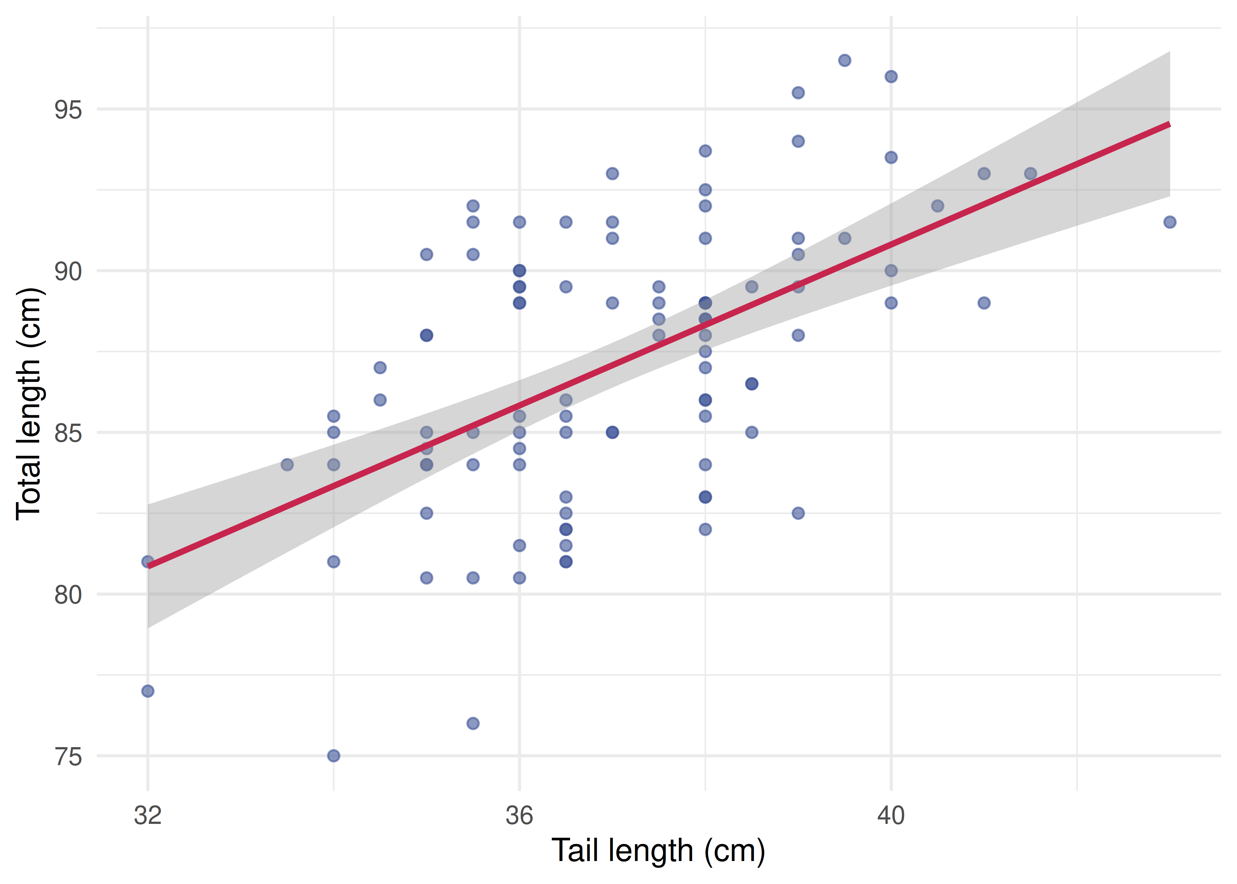
ggplot(possum, aes(tail_l, total_l)) +
  geom_point(alpha = 0.6, color = "#3E5496") +
  geom_smooth(method = "lm", se = TRUE, color = "#C7254E") +
  labs(x = "Tail length (cm)", y = "Total length (cm)") +
  theme_minimal(base_size = 13)

Total body length vs. tail length for 104 brushtail possums, with the least-squares line.

Note

Reading the permutation p-value. The relationship is strong enough that none of the shuffled slopes reaches the observed slope, so the simulation returns a p-value of 0. Report that honestly as p < 0.001 (smaller than \(1/\text{reps}\)) — very strong evidence — not literally zero.

Your deliverable

Submit a short report containing all of:

1. Graphic — a labeled scatterplot of total_l vs. tail_l with the fitted line.
2. Numerical result — the regression equation (intercept and slope), the slope’s p-value, and \(R^2\).
3. Interpret the slope — one sentence in context: how much does predicted total length change per extra cm of tail?
4. Conclusion in context — 3–4 sentences: is the slope discernibly different from 0? How strong is the relationship (\(R^2\))? Would you trust a prediction for a tail length far outside the observed range (extrapolation)?
5. One limitation — e.g., one species/region; correlation here is descriptive, not causal.

How it’s graded

Criterion	What we look for
Appropriate, labeled graphic	scatterplot with fitted line, axes labeled
Procedure & conditions	regression + slope test identified; residuals considered
Correct numerical result	equation, slope p-value, \(R^2\) reported correctly
Conclusion in context	slope interpreted; discernibility; no extrapolation
Communication	clear, correct interpretation

Warm up first. Fit a line by eye and see the residuals in the Regression explorer before writing your report.