15 Chi-Square Goodness of Fit
In previous chapters, we have developed inferential methods for comparing proportions across two groups. But what if we want to assess whether a single categorical variable with multiple levels follows a particular distribution? For instance, we might want to know if a jury pool is racially representative of the community, or whether the days of the week on which accidents occur are equally likely. The chi-square goodness of fit test is designed for exactly this purpose. It compares a set of observed counts to a set of expected counts derived from a hypothesized distribution, using a single test statistic that summarizes all of the differences at once.
15.1 Observed versus expected counts
Consider data from a random sample of 275 jurors in a small county. Jurors identified their racial group, and we would like to determine if these jurors are racially representative of the county’s population of registered voters. The observed counts and the population proportions are shown below.
| White | Black | Hispanic | Other | Total | |
|---|---|---|---|---|---|
| Observed jurors | 205 | 26 | 25 | 19 | 275 |
| Population proportion | 0.72 | 0.07 | 0.12 | 0.09 | 1.00 |
While the proportions in the jury sample do not precisely match the population proportions, it is unclear whether these data provide convincing evidence that the sample is not representative. If the jurors really were randomly sampled from the registered voters, we might expect small differences due to chance. However, unusually large differences may provide convincing evidence that the juries were not representative.
15.1.1 Computing expected counts
If the jurors were randomly sampled from the population (i.e., if the null hypothesis is true), we would expect the sample proportions to roughly match the population proportions. The expected count for each category is found by multiplying the sample size by the hypothesized proportion for that category.
Of the 275 people who served on a jury, about how many would we expect to be White if jurors are randomly selected from the population? How many would we expect to be Black?
About 72% of the population is White, so we would expect about 72% of the jurors to be White: \(0.72 \times 275 = 198\). Similarly, we would expect about 7% of the jurors to be Black, which would correspond to about \(0.07 \times 275 = 19.25\) Black jurors.
Twelve percent of the population is Hispanic and 9% represent other races. How many of the 275 jurors would we expect to be Hispanic? How many from other races?
Show answer
We would expect \(0.12 \times 275 = 33\) Hispanic jurors and \(0.09 \times 275 = 24.75\) jurors from other races.The complete table of observed and expected counts is:
| White | Black | Hispanic | Other | Total | |
|---|---|---|---|---|---|
| Observed counts | 205 | 26 | 25 | 19 | 275 |
| Expected counts | 198 | 19.25 | 33 | 24.75 | 275 |
Computing expected counts for a goodness of fit test.
If the null hypothesis specifies proportions \(p_1, p_2, \ldots, p_k\) for \(k\) categories, and the total sample size is \(n\), then the expected count for category \(i\) is:
\[E_i = n \times p_i\]
15.1.2 Setting up hypotheses
The sample proportions from each racial group were not a precise match for the population proportions. We need to test whether the differences are strong enough to provide convincing evidence that the jurors are not a random sample. These ideas can be organized into hypotheses:
- \(H_0\): The jurors are a random sample from the population. The observed counts reflect natural sampling fluctuation.
- \(H_A\): The jurors are not randomly sampled from the population. There is bias in juror selection.
To evaluate these hypotheses, we need to quantify how different the observed counts are from the expected counts. Strong evidence for the alternative hypothesis would come in the form of unusually large deviations from what would be expected based on sampling variation alone.
15.2 The chi-square statistic
To build a test statistic, we first compute the standardized difference between each observed and expected count. For each category \(i\):
\[Z_i = \frac{O_i - E_i}{\sqrt{E_i}}\]
where \(O_i\) is the observed count and \(E_i\) is the expected count. The denominator \(\sqrt{E_i}\) serves as the standard error for the count.
For the jury data:
\[ \begin{aligned} Z_{\text{White}} &= \frac{205 - 198}{\sqrt{198}} = 0.50 \\ Z_{\text{Black}} &= \frac{26 - 19.25}{\sqrt{19.25}} = 1.54 \\ Z_{\text{Hispanic}} &= \frac{25 - 33}{\sqrt{33}} = -1.39 \\ Z_{\text{Other}} &= \frac{19 - 24.75}{\sqrt{24.75}} = -1.16 \end{aligned} \]
We would like to use a single test statistic to determine if these four standardized differences are unusually far from zero as a group. We do this by squaring each standardized difference and adding them up:
\[X^2 = Z_1^2 + Z_2^2 + Z_3^2 + Z_4^2 = 0.50^2 + 1.54^2 + (-1.39)^2 + (-1.16)^2 = 5.89\]
Squaring each standardized difference before adding them together does two things:
- Any standardized difference that is squared will be positive, so negative and positive deviations both contribute to the test statistic.
- Differences that are already unusual (e.g., a standardized difference of 2.5) become much larger after squaring, which gives them more weight.
Chi-square test statistic.
The chi-square test statistic is the sum of the squared standardized differences between observed and expected counts:
\[X^2 = \sum_{i=1}^{k} \frac{(O_i - E_i)^2}{E_i}\]
where the sum is over all \(k\) categories, \(O_i\) is the observed count in category \(i\), and \(E_i\) is the expected count in category \(i\) under the null hypothesis.
15.3 Simulation-based goodness of fit test
Before turning to the mathematical chi-square distribution, it is instructive to see how a simulation-based approach works for goodness of fit tests.
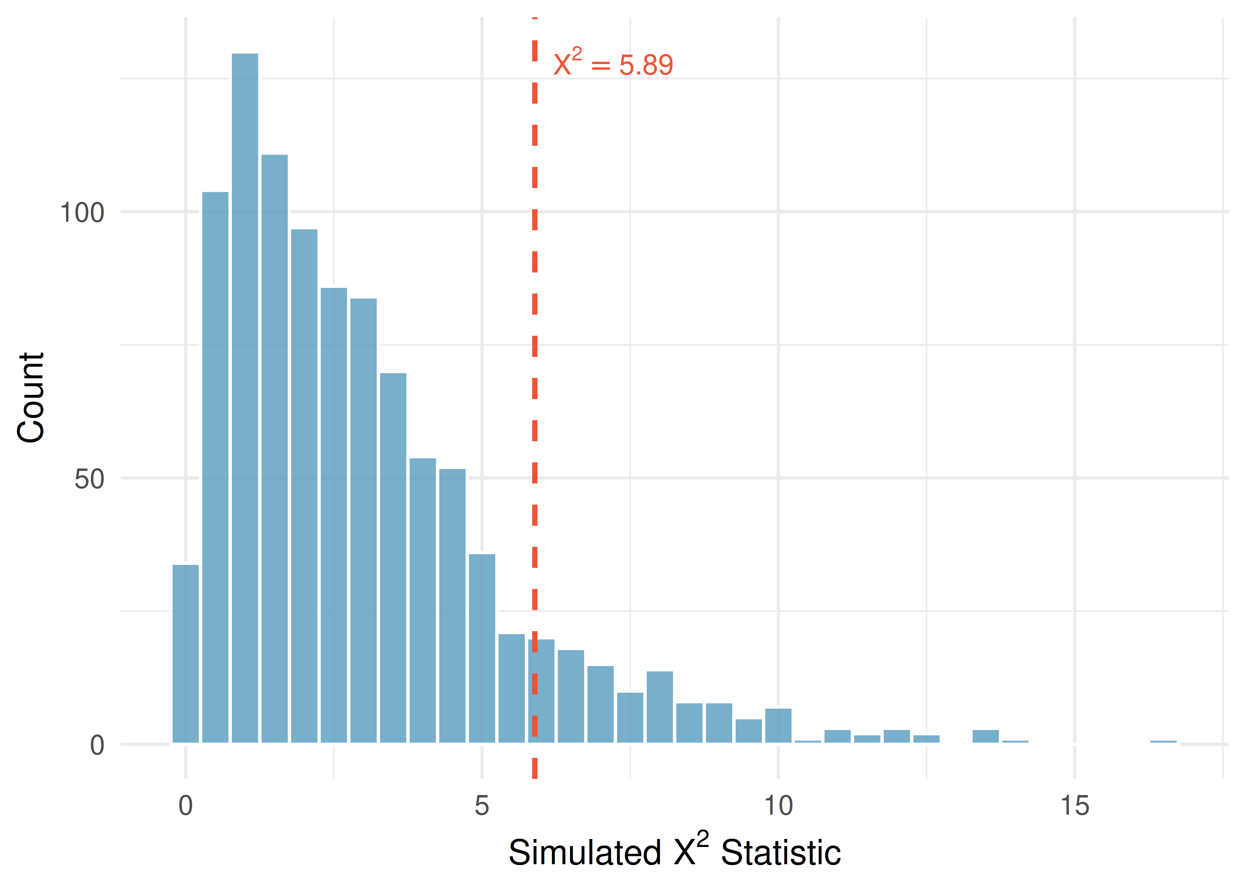
The idea is the same as in other randomization tests: if the null hypothesis is true (the data come from the hypothesized distribution), we can simulate many datasets that would arise under the null hypothesis and compute the chi-square statistic for each. This gives us a null distribution of the chi-square statistic, against which we can compare our observed statistic.
How the simulation works:
- Under \(H_0\), each observation has probability \(p_i\) of falling into category \(i\).
- For each simulated sample of size \(n\), randomly assign each observation to a category according to the null probabilities.
- Compute the chi-square statistic \(X^2\) for the simulated data.
- Repeat many times (e.g., 1,000 or 10,000 times) to build a null distribution.
- Compare the observed \(X^2\) to the null distribution. The \(p\)-value is the proportion of simulated statistics that are as large or larger than the observed statistic.
For the jury example, each simulated dataset would randomly assign 275 jurors to the four racial categories with probabilities 0.72, 0.07, 0.12, and 0.09. The resulting chi-square statistics from the simulated datasets form the null distribution.
The simulation-based approach confirms what we will find with the mathematical model: the observed chi-square statistic of 5.89 is not unusual enough to reject the null hypothesis at a 0.05 discernibility level.
See it in action. Open the Chi-Square GOF walkthrough for a guided pass through framing → checking expected counts → running the test → reading per-category contributions. Or open the Goodness-of-Fit Simulation to build the null χ² distribution by repeatedly drawing samples from the hypothesized distribution — a Predict → Do → Explain activity that lets you see why the mathematical chi-square curve is a reasonable model. For a bare tool, open the Goodness-of-Fit Test tool (analytic) or the Goodness-of-Fit Simulator (simulation) with the jury data preloaded, or enter your own data.
15.4 The chi-square distribution
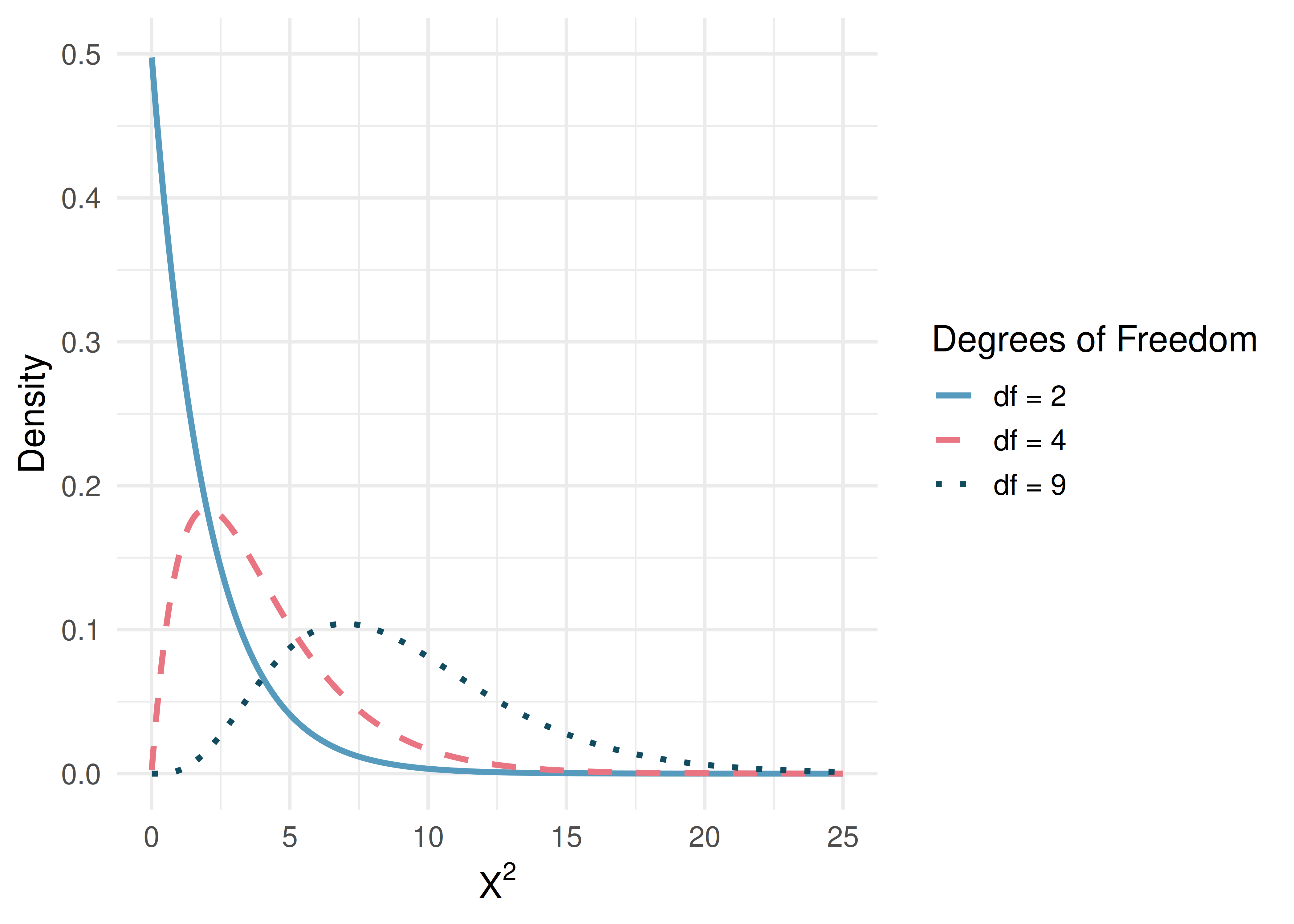
The chi-square test statistic \(X^2\) follows a chi-square distribution when the null hypothesis is true and the sample size conditions are met. The chi-square distribution is characterized by a single parameter called the degrees of freedom (df), which influences the shape, center, and spread of the distribution.
Key properties of the chi-square distribution:
- It is always non-negative (the chi-square statistic is a sum of squared values).
- It is right-skewed, especially for small degrees of freedom.
- As the degrees of freedom increase, the distribution becomes more symmetric and shifts to the right.
- The mean of the distribution equals the degrees of freedom.
15.4.1 Degrees of freedom for goodness of fit
For a goodness of fit test with \(k\) categories, the degrees of freedom are:
\[df = k - 1\]
How many categories were there in the juror example? How many degrees of freedom should be associated with the chi-square distribution?
There were \(k = 4\) categories: White, Black, Hispanic, and Other. The degrees of freedom are \(df = k - 1 = 3\).
15.5 Finding a \(p\)-value
If the null hypothesis is true, \(X^2\) follows a chi-square distribution with \(k - 1\) degrees of freedom. Because larger values of \(X^2\) correspond to greater deviations from the null hypothesis, the \(p\)-value is always found from the upper tail of the distribution.
For the jury data, the test statistic is \(X^2 = 5.89\) and the degrees of freedom are \(df = 3\). Find the \(p\)-value.
Using a chi-square distribution with 3 degrees of freedom, the area to the right of 5.89 is approximately 0.117.
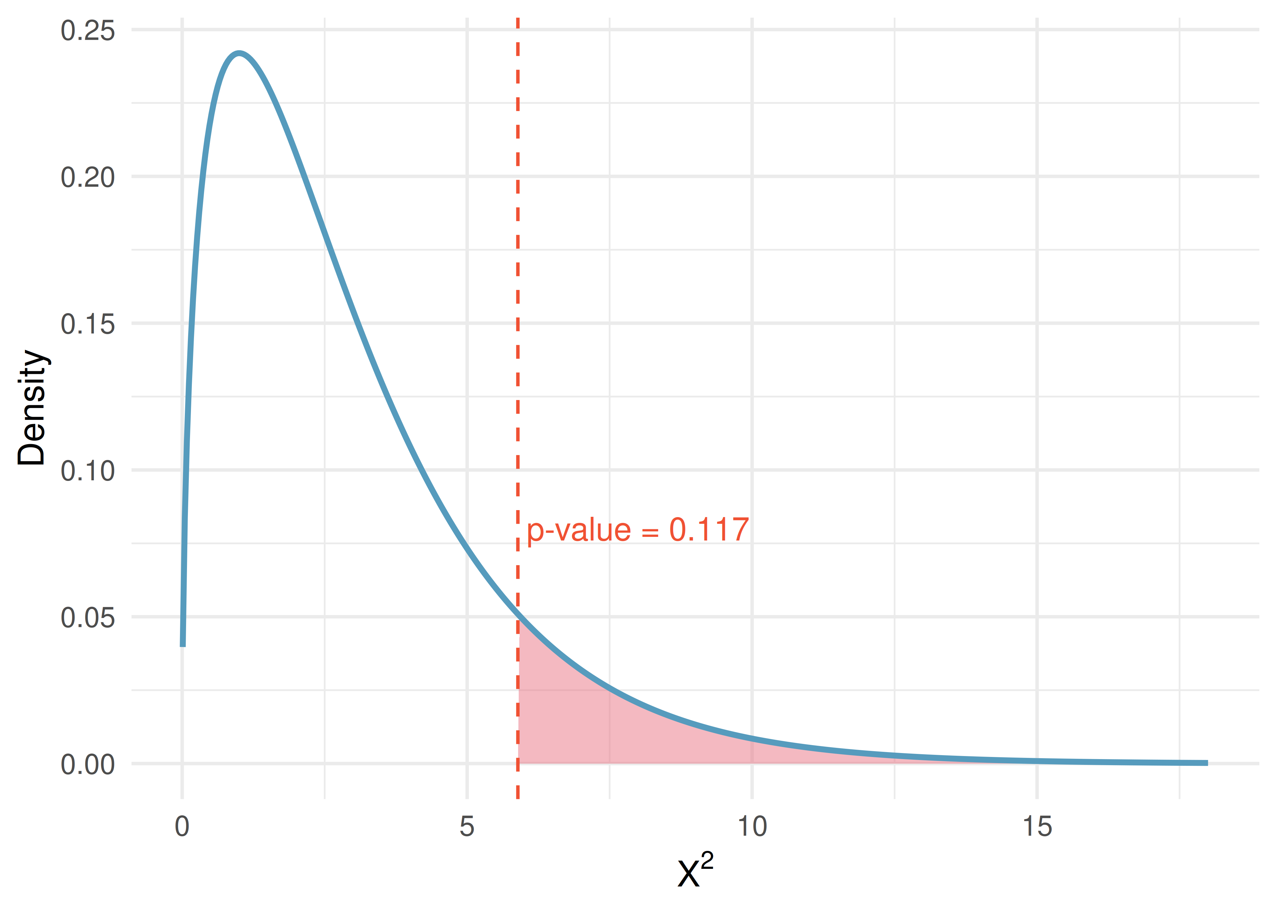
Since the \(p\)-value of 0.117 is larger than \(\alpha = 0.05\), we do not reject the null hypothesis. The data do not provide convincing evidence of racial bias in the juror selection process.
Consider a chi-square distribution with 5 degrees of freedom and a test statistic of 5.1. Find the \(p\)-value.
Using statistical software or a chi-square table, the area to the right of 5.1 on a chi-square distribution with 5 degrees of freedom is approximately 0.404. This is a very large \(p\)-value, so we would not reject the null hypothesis.
A chi-square distribution with 4 degrees of freedom has a test statistic of 10. Find the approximate \(p\)-value.
Show answer
Using statistical software, the area to the right of 10 on a chi-square distribution with 4 degrees of freedom is approximately 0.040. Since this is less than 0.05, we would reject the null hypothesis.15.6 Chi-square goodness of fit test
We can now summarize the complete procedure for a chi-square goodness of fit test.
Chi-square test for goodness of fit.
Suppose we want to evaluate whether the observed counts \(O_1, O_2, \ldots, O_k\) in \(k\) categories are consistent with a hypothesized distribution that specifies expected counts \(E_1, E_2, \ldots, E_k\).
Hypotheses:
- \(H_0\): The data follow the hypothesized distribution (the observed counts are consistent with the expected counts, up to sampling variability).
- \(H_A\): The data do not follow the hypothesized distribution.
Test statistic:
\[X^2 = \sum_{i=1}^{k} \frac{(O_i - E_i)^2}{E_i}\]
When the null hypothesis is true and the conditions are met, \(X^2\) follows a chi-square distribution with \(df = k - 1\).
The \(p\)-value is found from the upper tail of the chi-square distribution.
Conditions:
- Independence. Each case that contributes a count must be independent of all other cases.
- Sample size. Each expected count must be at least 5.
15.7 Evaluating goodness of fit for a distribution
The goodness of fit test can also be used to evaluate whether data follow a particular theoretical distribution.
Using 10 years of daily data for the S&P 500 stock index, we label each trading day as Up or Down and record how many days we must wait for each Up day: if the index rises on the next trading day, the wait is 1 day; if it falls once and then rises, the wait is 2 days; and so on. This gives 1,362 waiting times. We compare their observed frequencies to what we would expect if each day’s movement were independent of previous days, with the same chance of an Up day each day (a geometric distribution model). The observed and expected counts are shown below.
| Days until an Up day | 1 | 2 | 3 | 4 | 5 | 6 | 7+ |
|---|---|---|---|---|---|---|---|
| Observed | 717 | 369 | 155 | 69 | 28 | 14 | 10 |
| Expected | 743 | 338 | 154 | 70 | 32 | 14 | 12 |
Are these data consistent with the geometric distribution model?
We set up the hypotheses:
- \(H_0\): Stock returns are independent from one day to the next and follow a geometric model.
- \(H_A\): Stock returns show a pattern inconsistent with the geometric model.
The chi-square statistic is:
\[X^2 = \frac{(717 - 743)^2}{743} + \frac{(369 - 338)^2}{338} + \frac{(155 - 154)^2}{154} + \frac{(69 - 70)^2}{70} + \frac{(28 - 32)^2}{32} + \frac{(14 - 14)^2}{14} + \frac{(10 - 12)^2}{12} = 4.61\]
With \(k = 7\) categories, \(df = 6\). The \(p\)-value for \(X^2 = 4.61\) with 6 degrees of freedom is approximately 0.595.
Since the \(p\)-value is very large, we do not reject the null hypothesis. The data are consistent with the geometric distribution model, suggesting that stock movements may be independent from day to day over this period.
15.8 Chapter review
15.8.1 Summary
In this chapter, we developed the chi-square goodness of fit test, which assesses whether a sample of categorical data is consistent with a hypothesized distribution. The test uses the chi-square statistic, which measures how far the observed counts deviate from the expected counts. When the null hypothesis is true and the conditions are met, this statistic follows a chi-square distribution with \(k - 1\) degrees of freedom, where \(k\) is the number of categories. The \(p\)-value is always computed from the upper tail of the chi-square distribution, since larger values indicate greater discrepancy between the observed and expected counts.
15.8.2 Key terms
- Expected count
- Chi-square statistic (\(X^2\))
- Chi-square distribution
- Degrees of freedom (goodness of fit)
- Goodness of fit test
15.9 Exercises
- True or false, Part I. Determine if the statements below are true or false. For each false statement, suggest an alternative wording to make it a true statement.
The chi-square distribution, just like the normal distribution, has two parameters, mean and standard deviation.
The chi-square distribution is always right skewed, regardless of the value of the degrees of freedom parameter.
The chi-square statistic is always positive.
As the degrees of freedom increases, the shape of the chi-square distribution becomes more skewed.
- True or false, Part II. Determine if the statements below are true or false. For each false statement, suggest an alternative wording to make it a true statement.
As the degrees of freedom increases, the mean of the chi-square distribution increases.
If you found \(\chi^2 = 10\) with \(df = 5\) you would fail to reject \(H_0\) at the 5% significance level.
When finding the p-value of a chi-square test, we always shade the tail areas in both tails.
As the degrees of freedom increases, the variability of the chi-square distribution decreases.
- Open source textbook. A professor using an open source introductory statistics book predicts that 60% of the students will purchase a hard copy of the book, 25% will print it out from the web, and 15% will read it online. At the end of the semester he asks his students to complete a survey where they indicate what format of the book they used. Of the 126 students, 71 said they bought a hard copy of the book, 30 said they printed it out from the web, and 25 said they read it online.
State the hypotheses for testing if the professor’s predictions were inaccurate.
How many students did the professor expect to buy the book, print the book, and read the book exclusively online?
This is an appropriate setting for a chi-square test. List the conditions required for a test and verify they are satisfied.
Calculate the chi-squared statistic, the degrees of freedom associated with it, and the p-value.
Based on the p-value calculated in part (d), what is the conclusion of the hypothesis test? Interpret your conclusion in this context.
- Barking deer. Microhabitat factors associated with forage and bed sites of barking deer in Hainan Island, China were examined. In this region woods make up 4.8% of the land, cultivated grass plot makes up 14.7%, and deciduous forests make up 39.6%. Of the 426 sites where the deer forage, 4 were categorized as woods, 16 as cultivated grassplot, and 61 as deciduous forests. The table below summarizes these data.
Woods | Cultivated grassplot | Deciduous forests | Other | Total |
Write the hypotheses for testing if barking deer prefer to forage in certain habitats over others.
What type of test can we use to answer this research question?
Check if the assumptions and conditions required for this test are satisfied.
Do these data provide convincing evidence that barking deer prefer to forage in certain habitats over others? Conduct an appropriate hypothesis test to answer this research question.
StatLens Exercises
Let StatLens do the arithmetic; spend your effort on the reasoning a calculator can’t do.
Frame the question. A candy company claims that its mixed-color bag contains 30% red, 20% orange, 20% yellow, 15% green, and 15% blue candies. A consumer group buys one large bag and counts \(n = 400\) candies.
- What is the parameter framework here — a single proportion, several proportions, or a distribution across categories?
- Write the null and alternative hypotheses for the goodness-of-fit test in words and in symbols.
- Why is the GOF alternative always two-sided in spirit (there is no “one-sided” GOF)?
Choose the procedure. For each scenario, name the procedure — \(\chi^2\) goodness-of-fit, \(\chi^2\) test of independence, one-proportion \(z\), or not a chi-square problem.
- Does the distribution of M&M colors in a bag match the manufacturer’s claim?
- Is the gender distribution of voters (male/female/other) the same across three counties?
- Is the proportion of left-handed students at one school different from the national 10% rate?
- Are college majors (5 categories) independent of state of origin (4 categories)?
- Does birthday fall uniformly across the 12 months in a sample of 500 people?
Check conditions before you trust the test. Open the Goodness-of-Fit Test tool and enter (or load) a small dataset with at least one expected count below 5.
- What is the expected-count condition for the \(\chi^2\) GOF test? Why is it stated in terms of expected (not observed) counts?
- If one expected count is 3, should you trust the \(\chi^2\) p-value? What can you do instead — and what is the underlying issue with the \(\chi^2\) approximation in this regime?
- Suppose you have 10 categories and one expected count is 4. Can you simply merge the small-expected category with a neighbor? What is gained and what is lost by doing so?
Run it and interpret it. Open the Goodness-of-Fit Test tool and enter a five-category dataset (e.g., the candy bag).
Report the \(\chi^2\) statistic, degrees of freedom, and p-value.
State your decision at \(\alpha = 0.05\) and write a one-sentence conclusion in context.
The tool reports observed vs. expected counts for each category. Suppose \(H_0\) is rejected — how do you tell which categories drove the rejection? What does a large positive “observed \(-\) expected” residual for one category tell you?
Which statement is the correct interpretation of a p-value of 0.02?
- There is a 2% probability that the candy distribution matches the manufacturer’s claim.
- If the manufacturer’s claim were true, we would see a fit at least this bad about 2% of the time by chance.
- About 2% of candies in this bag came out wrong.
Simulation as a sanity check. Open the Goodness-of-Fit Simulator on the same dataset. (This tool draws repeated samples from the hypothesized distribution and builds the null \(\chi^2\) distribution empirically — the correct simulation analog for a GOF test.)
- Run 5000 simulated \(\chi^2\) statistics under \(H_0\). What does the null distribution look like — shape, support, where the observed \(\chi^2\) falls?
- Compare the simulation p-value to the \(\chi^2\) approximation p-value from Exercise 4. How close are they?
- Now repeat on a small dataset where at least one expected count is below 5. Are the two p-values still close? Which one would you trust, and why?
- A student says: “If the simulation and the formula agree, the simulation is redundant; if they disagree, the simulation is wrong.” Why is this exactly backwards?