11  Normal Approximation

In the randomization tests and bootstrap confidence intervals chapters, we used simulation-based methods to make inferences about population parameters. Those methods are powerful and flexible, but they share a limitation: every new problem requires running thousands of simulations. In this chapter, we introduce the normal distribution, a mathematical model that describes the bell-shaped pattern we keep seeing in our sampling distributions. When certain conditions are met, the normal distribution lets us calculate probabilities and construct confidence intervals using formulas instead of simulations. This is not a replacement for simulation-based thinking – it is a complement. The normal model provides the theoretical justification for why those simulations work the way they do.

11.1 The normal distribution

Among all the distributions encountered in statistics, one is overwhelmingly the most common. The symmetric, unimodal, bell-shaped curve is so ubiquitous that it goes by many names: the normal curve, the normal model, or the normal distribution.

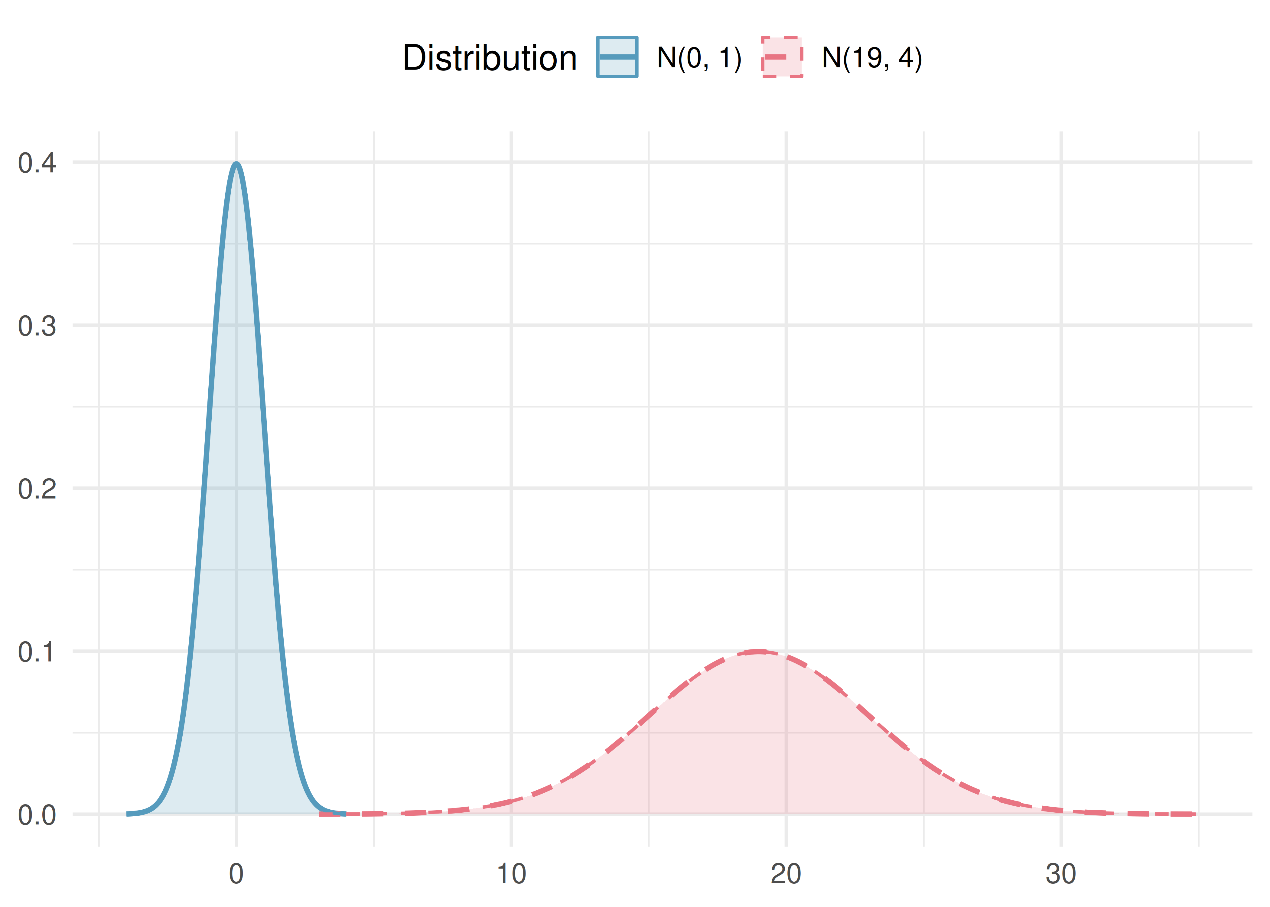
The normal distribution is a symmetric, unimodal, bell-shaped distribution described by two parameters: the mean \(\mu\) (which determines the center) and the standard deviation \(\sigma\) (which determines the spread). We write the distribution in shorthand as \(N(\mu, \sigma)\).

Figure 11.1: Two normal distributions with different parameters. The left curve has μ = 0 and σ = 1; the right curve has μ = 19 and σ = 4. Changing μ shifts the curve left or right; changing σ stretches or compresses it. ↗ Try this live — vary μ and σ and watch the curve slide and rescale.

Key properties of the normal distribution:

• The curve is perfectly symmetric about the mean \(\mu\).
• The total area under the curve is exactly 1 (representing 100% of observations). We can interpret any area under the curve as a proportion — and, equivalently, as the probability of a randomly selected observation falling in that range.
• The tails extend infinitely in both directions but get very close to zero far from the center.
• Changing \(\mu\) shifts the entire curve left or right without changing its shape.
• Increasing \(\sigma\) makes the curve wider and shorter; decreasing \(\sigma\) makes it narrower and taller.

Normal distribution facts. Many variables are nearly normal, but none are exactly normal. The normal distribution, while not perfect for any single problem, is extremely useful for a wide variety of problems. Variables like SAT scores, adult heights, and blood pressure measurements closely follow the normal distribution.

11.1.1 The standard normal distribution

The normal distribution with mean \(\mu = 0\) and standard deviation \(\sigma = 1\) is called the standard normal distribution, written \(N(0, 1)\). It serves as a reference distribution that we will use throughout the course.

Write down the shorthand for a normal distribution with each set of parameters.

1. Mean 5 and standard deviation 3
2. Mean \(-100\) and standard deviation 10
3. Mean 2 and standard deviation 9

---

1. \(N(\mu = 5, \sigma = 3)\)
2. \(N(\mu = -100, \sigma = 10)\)
3. \(N(\mu = 2, \sigma = 9)\)

11.2 The 68-95-99.7 rule

One of the most useful facts about the normal distribution is how observations spread out around the mean. This relationship is captured by the 68-95-99.7 rule (sometimes called the empirical rule).

The 68-95-99.7 rule. For any normal distribution \(N(\mu, \sigma)\):

• About 68% of observations fall within 1 standard deviation of the mean: between \(\mu - \sigma\) and \(\mu + \sigma\).
• About 95% of observations fall within 2 standard deviations of the mean: between \(\mu - 2\sigma\) and \(\mu + 2\sigma\).
• About 99.7% of observations fall within 3 standard deviations of the mean: between \(\mu - 3\sigma\) and \(\mu + 3\sigma\).

Figure 11.2: The 68-95-99.7 rule on a normal curve. About 68% of the area lies within μ ± σ, 95% within μ ± 2σ, and 99.7% within μ ± 3σ. Each labeled arrow bar spans exactly the region its percentage measures. ↗ Try this live — drag the cutlines to see the 68-95-99.7 boundaries live.

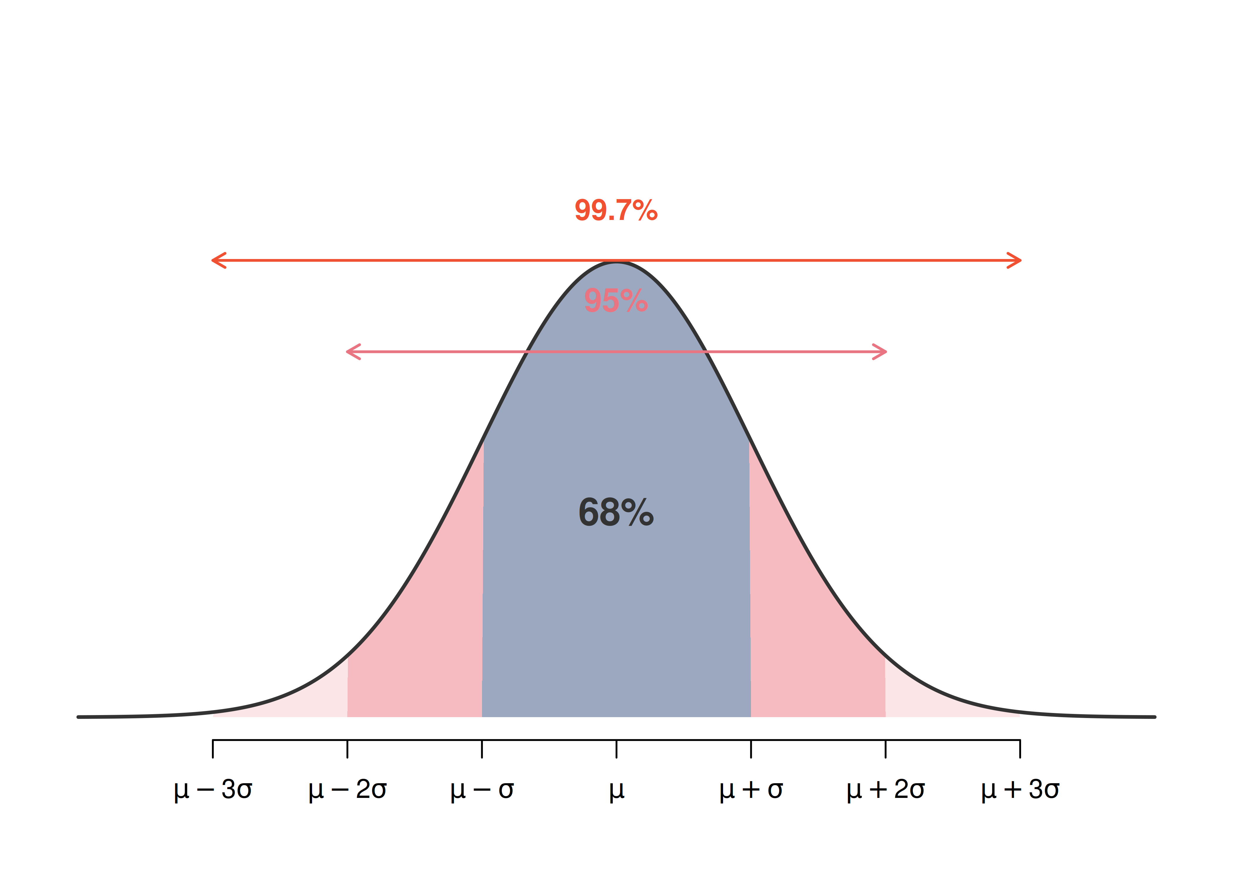
This rule gives quick, approximate answers without needing a calculator or software.

SAT scores closely follow the normal distribution with mean \(\mu = 1500\) and standard deviation \(\sigma = 300\).

1. About what percent of test takers score between 1200 and 1800?
2. About what percent score between 1500 and 2100?

---

1. 1200 is one standard deviation below the mean (\(1500 - 300 = 1200\)), and 1800 is one standard deviation above the mean (\(1500 + 300 = 1800\)). By the 68-95-99.7 rule, about 68% of test takers score between 1200 and 1800.

2. The range from 900 to 2100 covers \(\mu \pm 2\sigma\), which contains about 95% of scores. Since the normal distribution is symmetric, the range from 1500 to 2100 (the upper half) contains about \(\frac{95\%}{2} = 47.5\%\) of scores.

Adult male heights in the US follow approximately a normal distribution with mean 70 inches and standard deviation 3.3 inches. Using the 68-95-99.7 rule, approximately what percentage of adult males are between 63.4 and 76.6 inches tall?

Show answer

63.4 inches is \(70 - 2(3.3) = 63.4\) and 76.6 inches is \(70 + 2(3.3) = 76.6\). These are each 2 standard deviations from the mean, so by the 68-95-99.7 rule, approximately 95% of adult males have heights in this range.

Continuing with SAT scores (\(\mu = 1500\), \(\sigma = 300\)), about what percent of test takers score above 2100?

Show answer

2100 is 2 standard deviations above the mean. By the 68-95-99.7 rule, about 95% of scores are within 2 standard deviations, leaving about 5% outside. Since the distribution is symmetric, about 2.5% are above 2100.

11.3 Z-scores and standardizing

When comparing observations from different distributions, raw values are not directly comparable. A score of 1800 on the SAT and a score of 24 on the ACT look very different, but we need a common scale to determine which performance is better relative to other test takers. The solution is standardizing the observations.

The Z-score of an observation \(x\) from a distribution with mean \(\mu\) and standard deviation \(\sigma\) is the number of standard deviations it falls above or below the mean:

\[Z = \frac{x - \mu}{\sigma}\]

• Positive Z-scores indicate observations above the mean.
• Negative Z-scores indicate observations below the mean.
• A Z-score of 0 means the observation equals the mean.

If the observation \(x\) comes from a normal distribution \(N(\mu, \sigma)\), then its Z-score follows the standard normal distribution \(N(0, 1)\). Standardizing shifts the center to 0 and rescales the spread to 1, but preserves the normal shape.

SAT scores follow \(N(\mu = 1500, \sigma = 300)\) and ACT scores follow \(N(\mu = 21, \sigma = 5)\). Nel scored 1800 on the SAT and Sian scored 24 on the ACT. Who performed better relative to other test takers?

---

We compute Z-scores for each student.

Nel’s Z-score: \(Z_{\text{Nel}} = \frac{1800 - 1500}{300} = \frac{300}{300} = 1.00\)

Sian’s Z-score: \(Z_{\text{Sian}} = \frac{24 - 21}{5} = \frac{3}{5} = 0.60\)

Nel is 1 standard deviation above the SAT mean, while Sian is only 0.6 standard deviations above the ACT mean. Nel performed better relative to other test takers.

Head lengths of brushtail possums follow a nearly normal distribution with mean 92.6 mm and standard deviation 3.6 mm. Compute the Z-scores for possums with head lengths of 95.4 mm and 85.8 mm. Which possum has the more unusual head length?

Show answer

For \(x_1 = 95.4\) mm: \(Z_1 = \frac{95.4 - 92.6}{3.6} = \frac{2.8}{3.6} = 0.78\). For \(x_2 = 85.8\) mm: \(Z_2 = \frac{85.8 - 92.6}{3.6} = \frac{-6.8}{3.6} = -1.89\). The second possum has a more unusual head length because \(|{-1.89}| > |0.78|\).

Let \(X\) represent a value drawn at random from \(N(\mu = 3, \sigma = 2)\), and suppose we observe \(x = 5.19\).

1. Find the Z-score.
2. How many standard deviations above or below the mean is this observation?

---

1. \(Z = \frac{x - \mu}{\sigma} = \frac{5.19 - 3}{2} = \frac{2.19}{2} = 1.095\)

2. The observation is 1.095 standard deviations above the mean. We know it is above because the Z-score is positive.

11.4 Finding probabilities from the normal distribution

One of the most important skills in statistics is finding the probability that a normally distributed variable falls in a specified range. The idea is straightforward: area under the curve equals probability. You’ve already been doing this intuitively — in the randomization tests and bootstrap confidence intervals chapters, every time you counted “what fraction of simulated statistics were this extreme?” you were estimating a probability by looking at proportions in a distribution. The normal model just gives us a formula for the curve, so we can compute the area exactly instead of simulating it.

Strategy for normal probability problems. Always follow these steps:

1. Draw a picture. Sketch the normal curve, mark the mean, and shade the area you want to find.
2. Find the Z-score. Standardize the value(s) of interest using \(Z = \frac{x - \mu}{\sigma}\).
3. Look up the area. Use a normal probability table, statistical software, or the StatLens Normal Distribution Explorer to find the area to the left of the Z-score.
4. Adjust if needed. If you need a right-tail area, subtract the left-tail area from 1. For an area between two values, subtract the smaller left-tail area from the larger.

11.4.1 Left-tail probabilities (percentiles)

The area to the left of a value on the normal curve gives the percentile – the proportion of observations that fall below that value.

The percentile of an observation is the percentage of values in the distribution that fall at or below that observation.

Nel scored 1800 on the SAT (\(Z = 1.00\)). What percentile is this?

---

We need the area to the left of \(Z = 1.00\) on the standard normal curve.

Figure 11.3: The standard normal curve with the area to the left of Z = 1.00 shaded. This area represents Nel’s percentile. ↗ Try this live — drag the cutline to any Z value and read off the left-tail area.

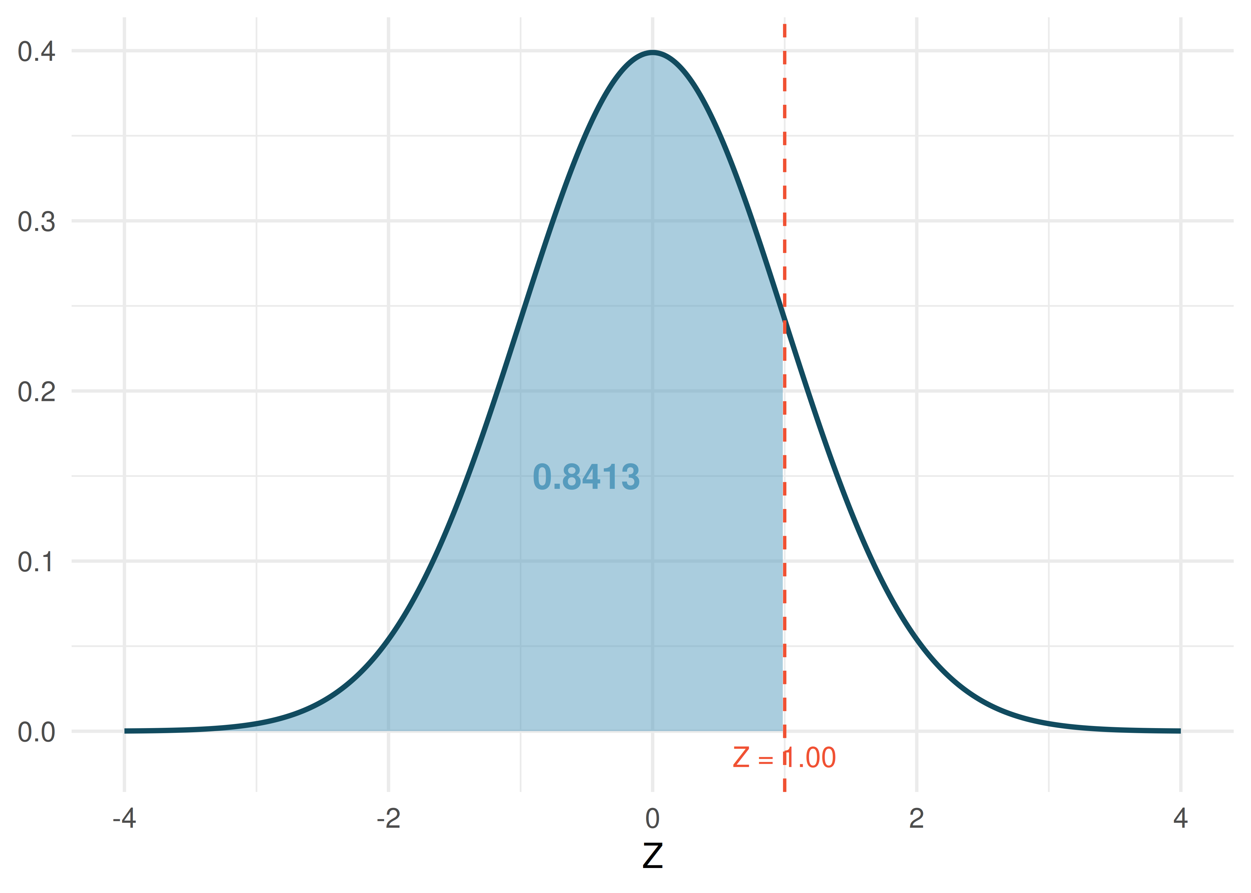
Using a normal probability table or software, the area to the left of \(Z = 1.00\) is 0.8413. Nel is at the 84th percentile – 84.13% of SAT takers scored lower.

11.4.2 Right-tail probabilities

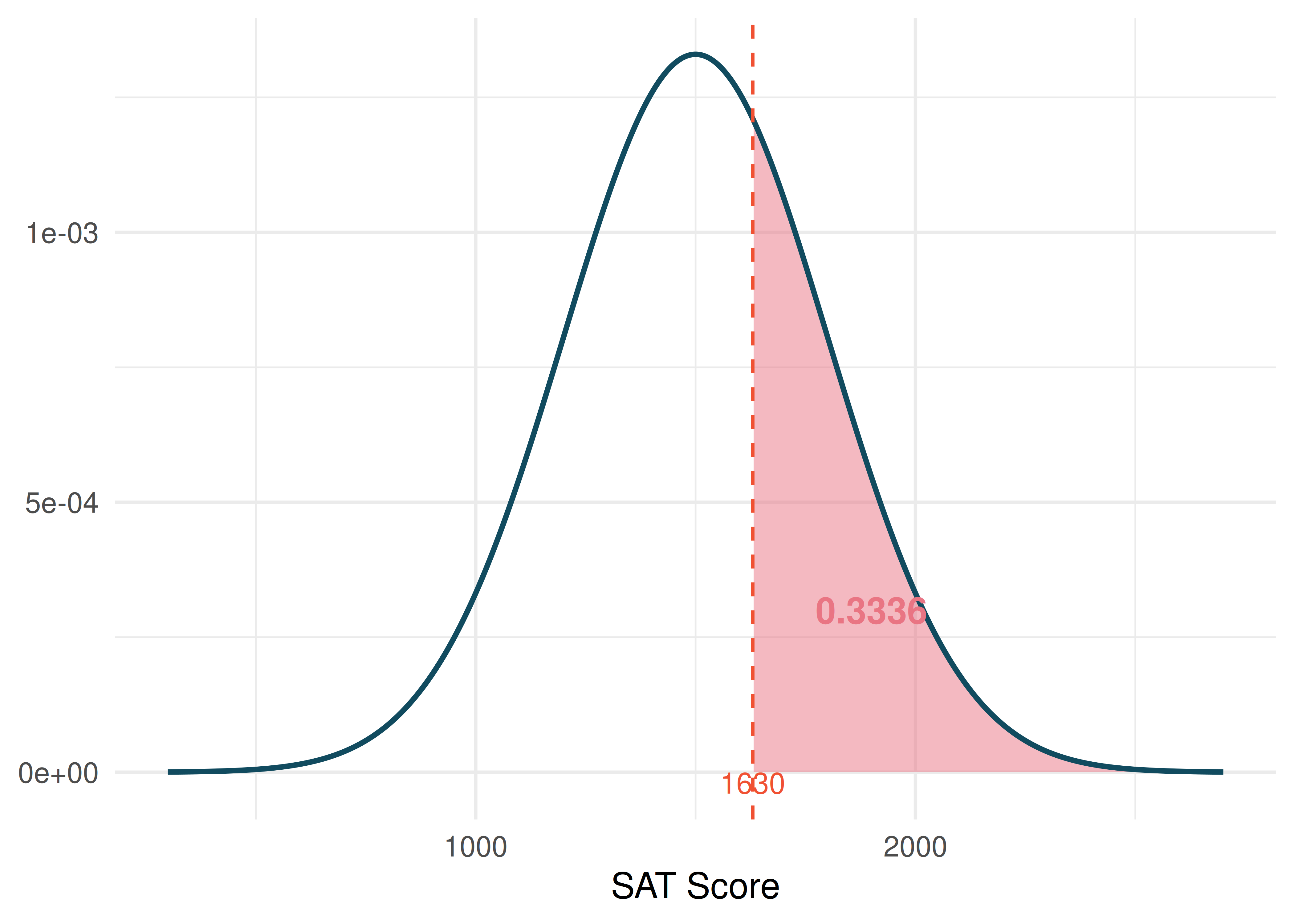
Shannon is a randomly selected SAT taker. What is the probability Shannon scores at least 1630?

---

Step 1: Draw a picture. We shade the area above 1630 on the \(N(1500, 300)\) curve.

Figure 11.4: A normal curve with mean 1500 and standard deviation 300. The area to the right of 1630 is shaded. ↗ Try this live — set μ, σ, and the cutline to reproduce this area.

Step 2: Find the Z-score.

\[Z = \frac{1630 - 1500}{300} = \frac{130}{300} = 0.43\]

Step 3: Look up the left-tail area. The area to the left of \(Z = 0.43\) is 0.6664.

Step 4: Adjust. The area to the right is \(1 - 0.6664 = 0.3336\).

The probability Shannon scores at least 1630 is 0.3336, or about 33.4%.

If the probability of Shannon scoring at least 1630 is 0.3336, what is the probability Shannon scores less than 1630?

Show answer

The probability of scoring less than 1630 is the area to the left: 0.6664, or about 66.6%. The left-tail and right-tail areas always sum to 1.

11.4.3 Probabilities between two values

Adult male heights follow \(N(\mu = 70, \sigma = 3.3)\) inches. What is the probability that a randomly selected adult male is between 5’9” (69 inches) and 6’2” (74 inches)?

---

Step 1: Draw a picture. Shade the area between 69 and 74 on the normal curve.

Figure 11.5: A normal curve centered at 70 with standard deviation 3.3. The area between 69 and 74 is shaded. ↗ Try this live — drag the two cutlines to shade any interval between them.

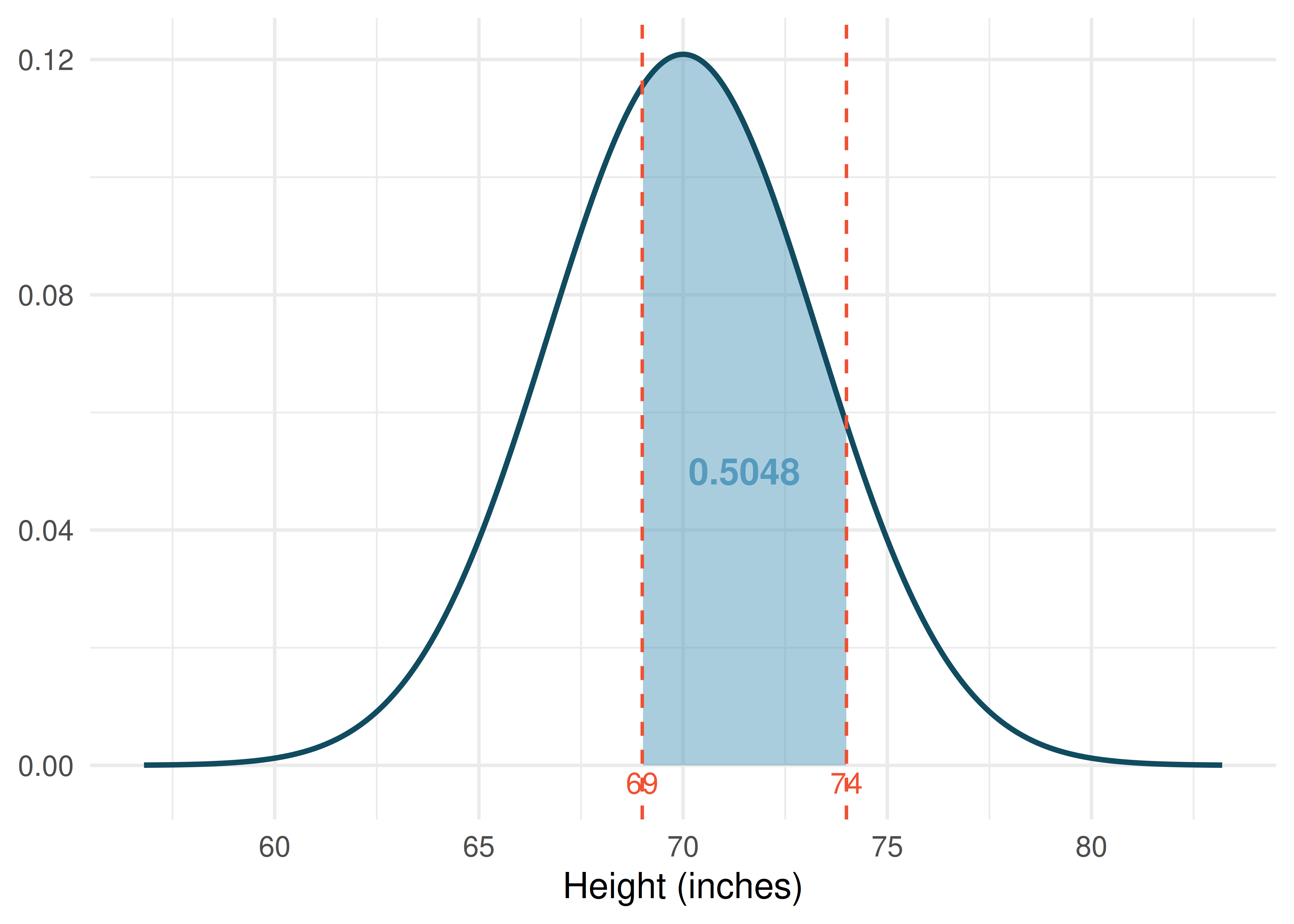
Step 2: Find both Z-scores.

\[Z_1 = \frac{69 - 70}{3.3} = -0.30 \qquad Z_2 = \frac{74 - 70}{3.3} = 1.21\]

Step 3: Look up both left-tail areas.

• Area to the left of \(Z_1 = -0.30\): 0.3821
• Area to the left of \(Z_2 = 1.21\): 0.8869

Step 4: Subtract.

\[P(69 < X < 74) = 0.8869 - 0.3821 = 0.5048\]

About 50.5% of adult males are between 5’9” and 6’2”.

What percent of SAT takers score between 1500 and 2000? (SAT scores follow \(N(1500, 300)\).)

Show answer

First find the Z-scores: \(Z_1 = \frac{1500 - 1500}{300} = 0.00\) and \(Z_2 = \frac{2000 - 1500}{300} = 1.67\). The left-tail areas are 0.5000 and 0.9525. The area between them is \(0.9525 - 0.5000 = 0.4525\), so about 45.25% score between 1500 and 2000.

11.4.4 Finding values from percentiles

Sometimes we want to work backwards: given a percentile, find the observation.

Adult male heights follow \(N(70, 3.3)\). Yousef’s height is at the 40th percentile. How tall is Yousef?

---

Step 1: Draw a picture. The 40th percentile means 40% of the area is to the left.

Step 2: Find the Z-score for the 40th percentile. Using a normal probability table (look for 0.40 in the body of the table) or software, \(Z = -0.25\).

Step 3: Solve for \(x\). Using the Z-score formula:

\[-0.25 = \frac{x - 70}{3.3}\]

\[x = 70 + (-0.25)(3.3) = 70 - 0.825 = 69.2 \text{ inches}\]

Yousef is approximately 69.2 inches (about 5’9”) tall.

What is the 95th percentile for SAT scores?

Show answer

The Z-score for the 95th percentile is \(Z = 1.645\). Then \(x = 1500 + 1.645 \times 300 = 1500 + 493.5 = 1993.5\). The 95th percentile for SAT scores is approximately 1994.

11.4.5 The normal probability table

A normal probability table (also called a Z-table) lists areas to the left of Z-scores for the standard normal distribution. The table is organized with the ones and tenths digits of the Z-score in the rows, and the hundredths digit in the columns.

Common Z-scores and areas worth remembering:

Commonly used Z-scores and their corresponding left-tail areas.

Z-score	Left-tail area	Interpretation
\(-1.96\)	0.0250	2.5th percentile
\(-1.645\)	0.0500	5th percentile
\(-1.00\)	0.1587	15.87th percentile
\(0.00\)	0.5000	50th percentile (the mean)
\(1.00\)	0.8413	84.13th percentile
\(1.645\)	0.9500	95th percentile
\(1.96\)	0.9750	97.5th percentile
\(2.576\)	0.9950	99.5th percentile

See it in action. Open the Normal Distribution Explorer to verify entries in the table above — enter a Z-score, check the shaded area, then work backwards from a percentile.

11.5 The normal approximation to sampling distributions

In the sampling distributions chapter, we used simulation to explore sampling distributions – the distributions of sample statistics computed from many repeated samples. A striking pattern emerged: regardless of whether we were looking at sample means, sample proportions, or differences in means or proportions, the sampling distributions tended to be bell-shaped and symmetric. This is not a coincidence.

11.5.1 The Central Limit Theorem

The Central Limit Theorem (CLT). When observations are independent and the sample size is sufficiently large, the sampling distribution of many common statistics (sample means, sample proportions, and their differences) is approximately normal, regardless of the shape of the population distribution.

Specifically:

• The sampling distribution of \(\bar{x}\) is approximately \(N\!\left(\mu, \frac{\sigma}{\sqrt{n}}\right)\).
• The sampling distribution of \(\hat{p}\) is approximately \(N\!\left(p, \sqrt{\frac{p(1-p)}{n}}\right)\).

The CLT is one of the most remarkable results in all of mathematics. It explains why simulation-based null distributions and bootstrap distributions looked bell-shaped: they were approximating the normal distribution all along.

Two conditions for the CLT to apply:

1. Independence. The observations must be independent of one another. This is satisfied when data come from a random sample or a randomized experiment.
2. Sample size. The sample must be large enough. What counts as “large enough” depends on the context:
   • For proportions: at least 10 expected successes and 10 expected failures (\(np \geq 10\) and \(n(1-p) \geq 10\)). This is called the success-failure condition.
   • For means: \(n \geq 30\) is a common guideline, though smaller samples can work if the population is not strongly skewed.

11.5.2 Standard error: quantifying the variability of a statistic

The CLT tells us the sampling distribution is approximately normal. But how wide is that normal distribution? The answer is given by the standard error.

The standard error (SE) of a statistic is the standard deviation of its sampling distribution. It measures how much the statistic varies from sample to sample.

The standard error depends on the parameter of interest:

Standard error formulas for common parameters.

Parameter	Point estimate	Standard error
Population mean \(\mu\)	\(\bar{x}\)	\(SE = \frac{s}{\sqrt{n}}\)
Population proportion \(p\)	\(\hat{p}\)	\(SE = \sqrt{\frac{\hat{p}(1-\hat{p})}{n}}\)
Difference in means \(\mu_1 - \mu_2\)	\(\bar{x}_1 - \bar{x}_2\)	\(SE = \sqrt{\frac{s_1^2}{n_1} + \frac{s_2^2}{n_2}}\)
Difference in proportions \(p_1 - p_2\)	\(\hat{p}_1 - \hat{p}_2\)	\(SE = \sqrt{\frac{\hat{p}_1(1-\hat{p}_1)}{n_1} + \frac{\hat{p}_2(1-\hat{p}_2)}{n_2}}\)

Margin of error. The distance \(z^* \times SE\) is called the margin of error. For a 95% confidence interval, \(z^* = 1.96\) (often rounded to 2), giving a margin of error of approximately \(2 \times SE\). This is directly connected to the 68-95-99.7 rule: 95% of sample statistics fall within about 2 standard errors of the true parameter value.

11.5.3 Connecting simulation and normal approximation

Let’s see the connection between simulation-based methods and the normal approximation in a concrete example. As a quick reminder from the randomization tests chapter, a hypothesis test weighs the null hypothesis \(H_0\) (“no effect”) against the alternative \(H_A\) (“real effect”), computes a p-value (probability of the observed data or more extreme under \(H_0\)), and rejects \(H_0\) when the p-value falls below the discernibility level \(\alpha\).

In the randomization tests chapter, we tested whether opportunity cost reminders reduce spending. We simulated 10,000 randomization samples and found a null distribution that was bell-shaped with a center of 0 and a spread described by \(SE \approx 0.078\). The observed difference was 0.20.

Simulation approach: Count how many of the 10,000 simulated differences were at least as extreme as 0.20. The proportion gives the p-value: approximately 0.006.

Normal approximation approach: Model the null distribution as \(N(0, 0.078)\). Compute the Z-score:

\[Z = \frac{0.20 - 0}{0.078} = 2.56\]

The area to the right of \(Z = 2.56\) is 0.0052.

Both approaches give nearly the same p-value (0.006 vs. 0.0052) and the same conclusion: reject \(H_0\). The normal approximation works because the conditions are met – independent observations and a sufficiently large sample.

11.5.4 Confidence intervals using the normal model

The normal approximation also lets us build confidence intervals without bootstrapping.

General confidence interval formula. When the sampling distribution of a statistic is approximately normal with standard error \(SE\), a confidence interval takes the form:

\[\text{point estimate} \pm z^* \times SE\]

where \(z^*\) is chosen based on the desired confidence level:

Critical values \(z^*\) for common confidence levels.

Confidence level	\(z^*\)
90%	1.645
95%	1.960
99%	2.576

A study examined whether stents reduce stroke risk. The observed difference in 30-day stroke rates (treatment minus control) was \(\hat{p}_T - \hat{p}_C = 0.090\), with \(SE = 0.028\). Construct a 95% confidence interval.

---

The conditions for the normal model have been verified. Using \(z^* = 1.96\):

\[0.090 \pm 1.96 \times 0.028 = 0.090 \pm 0.055 = (0.035, 0.145)\]

We are 95% confident that implanting a stent increased the 30-day stroke rate by between 3.5 and 14.5 percentage points. Since the interval does not contain 0, we have evidence of a real difference.

11.6 When does the normal model apply – and when doesn’t it?

The normal distribution is powerful but not universal. Here we summarize when it is and is not appropriate.

When the normal model is a good approximation:

• Sample proportions \(\hat{p}\), when the success-failure condition is met (\(np \geq 10\) and \(n(1-p) \geq 10\)).
• Sample means \(\bar{x}\), when the sample size is at least 30 or the population is approximately normal (we will use the \(t\)-distribution for means – see the confidence intervals for means chapter).
• Differences in proportions or means, when both groups satisfy the above conditions.

When the normal model is NOT a good approximation:

• Small samples with a skewed population distribution.
• Proportions near 0 or 1 with small sample sizes (the success-failure condition fails).
• Data with strong dependence between observations.

A medical consultant claims that only 3 of their 62 liver transplant clients had complications, compared to the national rate of 10%. Is it appropriate to use the normal approximation to test whether this consultant’s rate is lower?

---

Under the null hypothesis (\(p_0 = 0.10\)), we check the success-failure condition:

• Expected successes (complications): \(np_0 = 62 \times 0.10 = 6.2\)
• Expected failures (no complications): \(n(1 - p_0) = 62 \times 0.90 = 55.8\)

Since the expected number of successes (6.2) is less than 10, the success-failure condition is not met. The normal approximation would underestimate the variability and give an inaccurate p-value. A simulation-based approach (as in the randomization tests chapter) would be more appropriate here.

When conditions fail, use simulation. If the success-failure condition is not met or the sample size is too small for the normal approximation, we should fall back on the simulation-based methods from the randomization tests and bootstrap confidence intervals chapters. The bootstrap and randomization approaches work well even when the normal model does not. This is one of the great advantages of simulation-based inference: it is more broadly applicable.

11.7 Chapter review

11.7.1 Summary

This chapter introduced the normal distribution, the most commonly encountered distribution in statistics. Key concepts include:

• The normal distribution is described by two parameters: the mean \(\mu\) (center) and standard deviation \(\sigma\) (spread), written as \(N(\mu, \sigma)\).
• The 68-95-99.7 rule provides quick estimates: about 68%, 95%, and 99.7% of observations fall within 1, 2, and 3 standard deviations of the mean.
• A Z-score standardizes an observation by measuring how many standard deviations it lies from the mean: \(Z = \frac{x - \mu}{\sigma}\).
• Normal probabilities are found by computing Z-scores and looking up areas under the standard normal curve using tables, software, or StatLens.
• The Central Limit Theorem guarantees that sampling distributions of means and proportions are approximately normal when the sample is large enough and observations are independent.
• The standard error measures how much a statistic varies from sample to sample and is the key ingredient in confidence intervals and hypothesis tests.
• The normal approximation and simulation-based methods give similar results when conditions are met, but simulation is more flexible when conditions fail.

11.7.2 Key terms

Normal distribution, standard normal distribution, parameters (μ and σ), 68-95-99.7 rule, Z-score, standardizing, percentile, Central Limit Theorem (CLT), standard error (SE), margin of error, success-failure condition.

11.8 Exercises

Answers to odd-numbered exercises are provided in the Exercise Solutions appendix at the back of the book.

1. Chronic illness. In 2013, the Pew Research Foundation reported that “45% of U.S. adults report that they live with one or more chronic conditions”. However, this value was based on a sample, so it may not be a perfect estimate for the population parameter of interest on its own. The study reported a standard error of about 1.2%, and a normal model may reasonably be used in this setting.

1. Create a 95% confidence interval for the proportion of U.S. adults who live with one or more chronic conditions. Also interpret the confidence interval in the context of the study. (Pew Research Center 2013)

2. Identify each of the following statements as true or false. Provide an explanation to justify each of your answers.

   1. We can say with certainty that the confidence interval from part (a) contains the true percentage of U.S. adults who suffer from a chronic illness.

   2. If we repeated this study 1,000 times and constructed a 95% confidence interval for each study, then approximately 950 of those confidence intervals would contain the true fraction of U.S. adults who suffer from chronic illnesses.

   3. The poll provides statistically discernible evidence (at the \(\alpha = 0.05\) level) that the percentage of U.S. adults who suffer from chronic illnesses is below 50%.

   4. Since the standard error is 1.2%, only 1.2% of people in the study communicated uncertainty about their answer.

2. Social media users and news, mathematical model. A poll conducted in 2022 found that 50% of U.S. adults (i.e., a proportion of 0.5) get news from social media sometimes or often. The standard error for this estimate was 0.5% (i.e., 0.005), and a normal distribution may be used to model the sample proportion. (Pew Research Center 2022)

1. Construct a 99% confidence interval for the fraction of U.S. adults who get news on social media sometimes or often, and interpret the confidence interval in context.

2. Identify each of the following statements as true or false. Provide an explanation to justify each of your answers.

   1. The data provide statistically discernible evidence that more than half of U.S. adults users get news through social media sometimes or often. Use a discernibility level of \(\alpha = 0.01\).

   2. Since the standard error is 0.5%, we can conclude that 99.5% of all U.S. adults users were included in the study.

   3. If we want to reduce the standard error of the estimate, we should collect less data.

   4. If we construct a 90% confidence interval for the percentage of U.S. adults who get news through social media sometimes or often, the resulting confidence interval will be wider than a corresponding 99% confidence interval.

3. Interpreting a Z score from a sample proportion. Suppose that you conduct a hypothesis test about a population proportion and calculate the Z score to be 0.47. Which of the following is the best interpretation of this value? For the problems which are not a good interpretation, indicate the statistical idea being described.

1. The probability is 0.47 that the null hypothesis is true.

2. If the null hypothesis were true, the probability would be 0.47 of obtaining a sample proportion as far as observed from the hypothesized value of the population proportion.

3. The sample proportion is 0.47 standard errors greater than the hypothesized value of the population proportion.

4. The sample proportion is equal to 0.47 times the standard error.

5. The sample proportion is 0.47 away from the hypothesized value of the population.

6. The sample proportion is 0.47.

4. Mental health. The General Social Survey asked the question: “For how many days during the past 30 days was your mental health, which includes stress, depression, and problems with emotions, not good?” Based on responses from 1,151 US residents, the survey reported a 95% confidence interval of 3.40 to 4.24 days in 2010.

1. Interpret this interval in context of the data.

2. What does “95% confident” mean? Explain in the context of the application.

3. Suppose the researchers think a 99% confidence level would be more appropriate for this interval. Will this new interval be smaller or wider than the 95% confidence interval?

4. If a new survey were to be done with 500 Americans, do you think the standard error of the estimate be larger, smaller, or about the same.

5. Area under the curve, Part I. What percent of a standard normal distribution \(N(\mu=0, \sigma=1)\) is found in each region? Be sure to draw a graph.

1. \(Z < -1.35\)

2. \(Z > 1.48\)

3. \(-0.4 < Z < 1.5\)

4. \(|Z| > 2\)

6. Area under the curve, Part II. What percent of a standard normal distribution \(N(\mu=0, \sigma=1)\) is found in each region? Be sure to draw a graph.

1. \(Z > -1.13\)

2. \(Z < 0.18\)

3. \(Z > 8\)

4. \(|Z| < 0.5\)

7. GRE scores, Part I. Sophia who took the Graduate Record Examination (GRE) scored 160 on the Verbal Reasoning section and 157 on the Quantitative Reasoning section. The mean score for Verbal Reasoning section for all test takers was 151 with a standard deviation of 7, and the mean score for the Quantitative Reasoning was 153 with a standard deviation of 7.67. Suppose that both distributions are nearly normal.

1. Write down the short-hand for these two normal distributions.

2. What is Sophia’s Z-score on the Verbal Reasoning section? On the Quantitative Reasoning section? Draw a standard normal distribution curve and mark these two Z-scores.

3. What do these Z-scores tell you?

4. Relative to others, which section did she do better on?

5. Find her percentile scores for the two exams.

6. What percent of the test takers did better than her on the Verbal Reasoning section? On the Quantitative Reasoning section?

7. Explain why simply comparing raw scores from the two sections could lead to an incorrect conclusion as to which section a student did better on.

8. If the distributions of the scores on these exams are not nearly normal, would your answers to parts (b) - (f) change? Explain your reasoning.

8. Triathlon times, Part I. In triathlons, it is common for racers to be placed into age and gender groups. Friends Leo and Mary both completed the Hermosa Beach Triathlon, where Leo competed in the Men, Ages 30 - 34 group while Mary competed in the Women, Ages 25 - 29 group. Leo completed the race in 1:22:28 (4948 seconds), while Mary completed the race in 1:31:53 (5513 seconds). Obviously Leo finished faster, but they are curious about how they did within their respective groups. Can you help them? Here is some information on the performance of their groups:

• The finishing times of the Men, Ages 30 - 34 group has a mean of 4313 seconds with a standard deviation of 583 seconds.
• The finishing times of the Women, Ages 25 - 29 group has a mean of 5261 seconds with a standard deviation of 807 seconds.
• The distributions of finishing times for both groups are approximately Normal.

Remember: a better performance corresponds to a faster finish.

1. Write down the short-hand for these two normal distributions.

2. What are the Z-scores for Leo’s and Mary’s finishing times? What do these Z-scores tell you?

3. Did Leo or Mary rank better in their respective groups? Explain your reasoning.

4. What percent of the triathletes did Leo finish faster than in his group?

5. What percent of the triathletes did Mary finish faster than in her group?

6. If the distributions of finishing times are not nearly normal, would your answers to parts (b) - (e) change? Explain your reasoning.

9. GRE scores, Part II. In a previous exercise we saw two distributions for GRE scores: \(N(\mu=151, \sigma=7)\) for the verbal part of the exam and \(N(\mu=153, \sigma=7.67)\) for the quantitative part. Use this information to compute each of the following:

1. The score of a student who scored in the \(80^{th}\) percentile on the Quantitative Reasoning section.

2. The score of a student who scored worse than 70% of the test takers in the Verbal Reasoning section.

10. Triathlon times, Part II. In a previous exercise we saw two distributions for triathlon times: \(N(\mu=4313, \sigma=583)\) for Men, Ages 30 - 34 and \(N(\mu=5261, \sigma=807)\) for the Women, Ages 25 - 29 group. Times are listed in seconds. Use this information to compute each of the following:

1. The cutoff time for the fastest 5% of athletes in the men’s group, i.e. those who took the shortest 5% of time to finish.

2. The cutoff time for the slowest 10% of athletes in the women’s group.

11. LA weather, Part I. The average daily high temperature in June in LA is 77\(^\circ\) F with a standard deviation of 5\(^\circ\) F. Suppose that the temperatures in June closely follow a normal distribution.

1. What is the probability of observing an 83\(^\circ\) F temperature or higher in LA during a randomly chosen day in June?

2. How cool are the coldest 10% of the days (days with lowest high temperature) during June in LA?

12. CAPM. The Capital Asset Pricing Model (CAPM) is a financial model that assumes returns on a portfolio are normally distributed. Suppose a portfolio has an average annual return of 14.7% (i.e. an average gain of 14.7%) with a standard deviation of 33%. A return of 0% means the value of the portfolio doesn’t change, a negative return means that the portfolio loses money, and a positive return means that the portfolio gains money.

1. What percent of years does this portfolio lose money, i.e. have a return less than 0%?

2. What is the cutoff for the highest 15% of annual returns with this portfolio?

13. LA weather, Part II. A previous exercise states that average daily high temperature in June in LA is 77\(^\circ\) F with a standard deviation of 5\(^\circ\) F, and it can be assumed that they follow a normal distribution. We use the following equation to convert \(^\circ\) F (Fahrenheit) to \(^\circ\) C (Celsius): \[C = (F - 32) \times \frac{5}{9}.\]

1. Write the probability model for the distribution of temperature in \(^\circ\) C in June in LA.

2. What is the probability of observing a 28\(^\circ\) C (which roughly corresponds to 83\(^\circ\) F) temperature or higher in June in LA? Calculate using the \(^\circ\) C model from part (a).

3. Did you get the same answer or different answers in part (b) of this question and part (a) of a previous exercise? Are you surprised? Explain.

4. Estimate the IQR of the temperatures (in \(^\circ\) C) in June in LA.

14. Find the SD (seedling heights). Heights of seedlings in a greenhouse experiment are approximately normally distributed with mean 16 cm. The greenhouse classifies a seedling as “tall” when its height exceeds 20 cm, and about 15% of seedlings fall into that category.

1. What is the z-score corresponding to the “tall” cutoff?

2. Use the z-score and the cutoff to find the standard deviation of seedling heights.

3. Which step lets you solve for \(\sigma\) once the z-score is known?

15. Overlay: normal curve on a simulated sampling distribution. In a previous chapter you built the sampling distribution of \(\hat{p}\) by drawing many random samples from a population with proportion \(p\) and computing \(\hat{p}\) each time. Below are three simulated sampling distributions of \(\hat{p}\) for \(p = 0.30\), using 5,000 samples each. Each histogram has a normal curve \(N(\mu, \sigma)\) overlaid, with \(\mu = p = 0.30\) and \(\sigma = \sqrt{p(1-p)/n}\).

• Panel A: \(n = 10\)
• Panel B: \(n = 50\)
• Panel C: \(n = 200\)

(Imagine three histograms stacked, each with a smooth bell curve laid over it. At \(n = 10\) the histogram is chunky and the curve doesn’t hug it well, especially in the left tail near 0. At \(n = 50\) the histogram is smoother and the curve fits well through the middle, with only small mismatch at the tails. At \(n = 200\) the histogram and curve are nearly indistinguishable.)

1. In which panel does the normal curve fit the simulated sampling distribution best? Why?

2. In panel A (\(n = 10\)), name one visible reason the fit is poor. What condition from the chapter is failing?

3. The chapter states the success-failure condition (\(np \ge 10\) and \(n(1-p) \ge 10\)) for the normal approximation. Check the condition for each panel using \(p = 0.30\). Which panels satisfy it?

4. What does this tell you about why the normal approximation is a useful tool? What does it require to work?

16. Bridge: simulation p-value vs. normal-approximation p-value. In the randomization tests chapter, you tested for sex discrimination in a bank promotion study by shuffling promotion decisions many times and recording the difference in promotion rates between male and female applicants. The observed difference was \(\hat{p}_M - \hat{p}_F = 0.292\). Suppose the randomization distribution of the difference, based on 10,000 shuffles, was centered near 0 with a standard deviation of about 0.115, and 47 of the 10,000 shuffles produced a difference \(\ge 0.292\).

1. Compute the simulation p-value (one-tailed).

2. Now compute the normal-approximation p-value for the same test. Treat the randomization distribution as approximately \(N(0, 0.115)\) and compute the Z-score for the observed statistic \(0.292\); then use the tail probability under the standard normal (via technology).

3. Do the two p-values agree? Within what tolerance?

4. Under what conditions would you expect the two p-values to disagree? Name one situation where the simulation p-value would be more trustworthy.

StatLens Exercises

Let StatLens do the arithmetic; spend your effort on the reasoning a calculator can’t do.

1. Read a normal probability in plain English. Open the Normal Distribution tool preset to \(\mu = 0\), \(\sigma = 1\).

   1. Drag the boundary to \(z = 1\). Report the area to the right. What is the matching area to the left of \(z = -1\)? Why are they equal?
   2. Switch to the “middle” tail and set the boundaries to \(\pm 2\). What is the area? Is your answer consistent with the 68–95–99.7 rule?
   3. Switch back to “left tail” and set the boundary so the area is exactly 0.025. What \(z\)-value did you get? Where will you use this number later in the course?
   4. A student says: “Areas under the curve are probabilities, so they must be less than 1.” Could you have an area of 1? An area of 0? What do those represent?

2. Standardize, then read off the probability. SAT math scores are approximately \(N(\mu = 520, \sigma = 110)\).

   1. Compute the \(z\)-score for a student who scored 700.
   2. Use Normal at \(\mu = 520, \sigma = 110\) to find the proportion of test-takers scoring above 700.
   3. Now use the standardized normal at \(\mu = 0, \sigma = 1\) and set the boundary to your \(z\)-score from (a). Same answer?
   4. A counselor says: “About 5% of students score 700 or higher.” Explain in one sentence what is probabilistic about the 5% and what is not.

3. The sampling distribution of \(\bar{x}\) is also normal — with different \(\sigma\). Continuing the SAT example: a school selects a random sample of \(n = 25\) students and computes their mean math score \(\bar{x}\).

   1. What is the sampling distribution of \(\bar{x}\)? Give its mean, standard error, and shape.
   2. Use the appropriate normal tool (pre-loaded with \(\mu = 520\), \(\sigma = 110/\sqrt{25} = 22\)) to find the probability that \(\bar{x} \ge 550\).
   3. Compare this to the probability that an individual student scores \(\ge 550\). Which is bigger and why?
   4. The school doubles \(n\) to 50. Will the probability in (b) get bigger or smaller? Why?

4. Normal approximation to a proportion — when does the formula work? Open the One-Proportion \(z\)-Test tool.

   1. Enter a scenario where \(\hat{p}\) is close to 0.5 and \(n\) is large (say \(\hat{p} = 0.45\), \(n = 200\)). Run a test. The tool reports the success–failure counts. Does the normal approximation apply?
   2. Now enter a scenario with small \(\hat{p}\): \(\hat{p} = 0.05\), \(n = 40\). Does the normal approximation apply? Why or why not?
   3. For the small-\(\hat{p}\) scenario in (b), if the test gives a small p-value, should you trust it? What should you do instead?
   4. Why is the success–failure rule based on \(np_0\) and \(n(1 - p_0)\) (using the null \(p_0\)) rather than \(n\hat{p}\) and \(n(1 - \hat{p})\) for a hypothesis test?

5. Simulation vs. analytic — when does the normal model agree with the bootstrap? Pair the One-Proportion \(z\)-Test with the Bootstrap CI for One Proportion on two datasets.

   First a well-behaved case: any dataset with \(\hat{p}\) near 0.5 and \(n \ge 100\).

   1. Compare the 95% intervals from the two tools. How close are they?

   Now a troublesome case: a dataset with small \(\hat{p}\) (e.g., the medical consultant data, \(\hat{p} \approx 0.05\)).

   2. Compare the 95% intervals again. Where do they disagree — in the midpoint, the width, or both?
   3. Look at the bootstrap distribution of \(\hat{p}\). Is it symmetric or skewed? How does that explain the disagreement with the symmetric \(z\)-interval?
   4. A student says: “Both intervals are ‘right’ — they’re just approximations.” What’s a more accurate framing? Which interval is more honest in the troublesome case, and what does “honest” mean for an interval?

Pew Research Center. 2013. “The Diagnosis Difference.” https://www.openintro.org/go?id=textbook-pew-2013-diagnosis-difference.

———. 2022. “News Consumption Across Digital Platforms.” https://www.pewresearch.org/journalism/fact-sheet/news-platform-fact-sheet/pj_2022-09-20_news-platforms_0-03b/.