Project: Comparing Two Means

Project — Inference for Means. Carry out the analysis end to end in Jamovi (or R) and communicate the result as a short report. The graded skills are framing the comparison, checking conditions, and interpreting in context — not the arithmetic.

The question

Does a mother’s smoking during pregnancy relate to her baby’s birth weight?

Is the mean birth weight different for babies of smokers and nonsmokers?

The data

The ncbirths dataset records 1,000 births in North Carolina. You’ll use weight (birth weight, in pounds) and habit (smoker or nonsmoker). This is observational data — keep that in mind when you write the conclusion.

Plan it first

1. Parameter. Define \(\mu_1 - \mu_2\) in words (mean weight for nonsmokers minus mean weight for smokers).
2. Hypotheses. State \(H_0\) and \(H_A\) for “the mean birth weights differ.” One- or two-sided?
3. Procedure. Two independent groups, a numerical outcome → a two-sample \(t\) procedure. (It is not paired — different babies in each group.)
4. Conditions. Each group is large and the data are not wildly skewed, so the \(t\)-procedure is reasonable. What would you check to be sure?

Do the analysis

Jamovi

1. Open ncbirths.csv.
2. T-Tests → Independent Samples T-Test. Dependent variable: weight; Grouping variable: habit.
3. Request mean difference, confidence interval, and a descriptives table; turn on the normality and equality-of-variances checks.
4. Read off the group means, the difference, the confidence interval, and the p-value.

(Jamovi screenshots to be added.)

R

library(infer)
library(dplyr)
library(ggplot2)
library(openintro)
data(ncbirths)

# Keep rows with a recorded habit
d <- ncbirths |> filter(!is.na(habit))

# Group means, SDs, and sizes
d |>
  group_by(habit) |>
  summarize(mean = mean(weight), sd = sd(weight), n = n())

# A tibble: 2 × 4
  habit      mean    sd     n
  <fct>     <dbl> <dbl> <int>
1 nonsmoker  7.14  1.52   873
2 smoker     6.83  1.39   126

# Two-sample t-test with a 95% CI for the difference (infer)
d |> t_test(weight ~ habit, order = c("nonsmoker", "smoker"))

# A tibble: 1 × 7
  statistic  t_df p_value alternative estimate lower_ci upper_ci
      <dbl> <dbl>   <dbl> <chr>          <dbl>    <dbl>    <dbl>
1      2.36  171.  0.0195 two.sided      0.316   0.0515    0.580

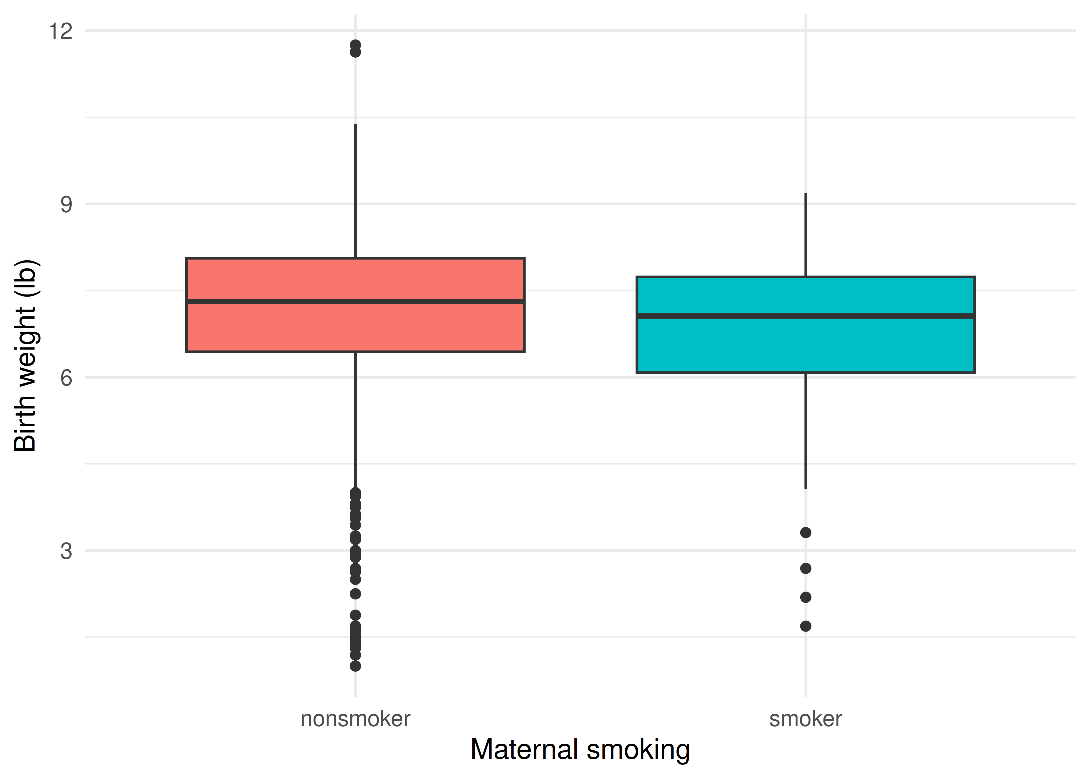
ggplot(d, aes(habit, weight, fill = habit)) +
  geom_boxplot(show.legend = FALSE) +
  labs(x = "Maternal smoking", y = "Birth weight (lb)") +
  theme_minimal(base_size = 13)

Birth weight by maternal smoking status. Babies of smokers weigh somewhat less on average.

Your deliverable

Submit a short report containing all of:

1. Graphic — labeled side-by-side boxplots of weight by habit.
2. Numerical result — the two group means, the difference, the 95% confidence interval, and the p-value.
3. Conditions — one sentence on why the two-sample \(t\) is reasonable here.
4. Conclusion in context — 3–4 sentences: is the difference discernible, in which direction, and — because this is observational — why you should not claim smoking causes the difference.
5. One limitation — e.g., confounding (smokers may differ in other ways), or self-reported smoking.

How it’s graded

Criterion	What we look for
Appropriate, labeled graphic	boxplots by group, axes labeled
Procedure & conditions	two-sample \(t\) identified; conditions addressed
Correct numerical result	means, difference, CI, p-value reported correctly
Conclusion in context	discernibility + direction + no causal claim (observational)
Communication	clear, correct interpretation

Warm up first. Try the same comparison in the Two-Means tool before writing your report.