14 Hypothesis Tests for Means
In the randomization tests chapter, we developed the logic of hypothesis testing using simulation: shuffle the data under the null hypothesis, build a null distribution, and measure how extreme the observed statistic is. In the confidence intervals for means chapter, we introduced the \(t\)-distribution as a mathematical model for the sampling distribution of means. Now we bring these ideas together. In this chapter, we use the \(t\)-distribution to conduct hypothesis tests for a single mean, the difference between two independent means, and the mean of paired differences. Along the way, we will see that the \(t\)-test and simulation-based tests generally agree when conditions are met, and we will discuss what to do when they disagree.
14.1 Testing a single mean by simulation
In the randomization tests chapter we tested a difference between two groups by shuffling the group labels, and in the inference for proportions chapter we tested a single proportion by drawing from a modeled null population — the marbles bag. A single mean needs its own version of that idea. There are no group labels to shuffle, and the data are numbers rather than successes and failures. But the goal is the same: build a world in which the null hypothesis is exactly true, then see how often chance alone produces a sample mean as extreme as the one we observed.
Suppose we want to test \(H_0: \mu = \mu_0\). Our sample mean \(\bar{x}\) almost certainly differs from \(\mu_0\) — the question is whether that difference is larger than sampling variability would produce if \(\mu_0\) really were the truth. We build the null world in two moves:
- Shift the data so its mean is exactly \(\mu_0\). Add the same constant to every value (whatever it takes to move \(\bar{x}\) onto \(\mu_0\)). This forces the null hypothesis to be true while leaving the data’s shape and spread untouched.
- Resample with replacement from the shifted data, many times, recording each resample’s mean. Those simulated means show how \(\bar{x}\) would bounce around from sample to sample if \(\mu = \mu_0\).
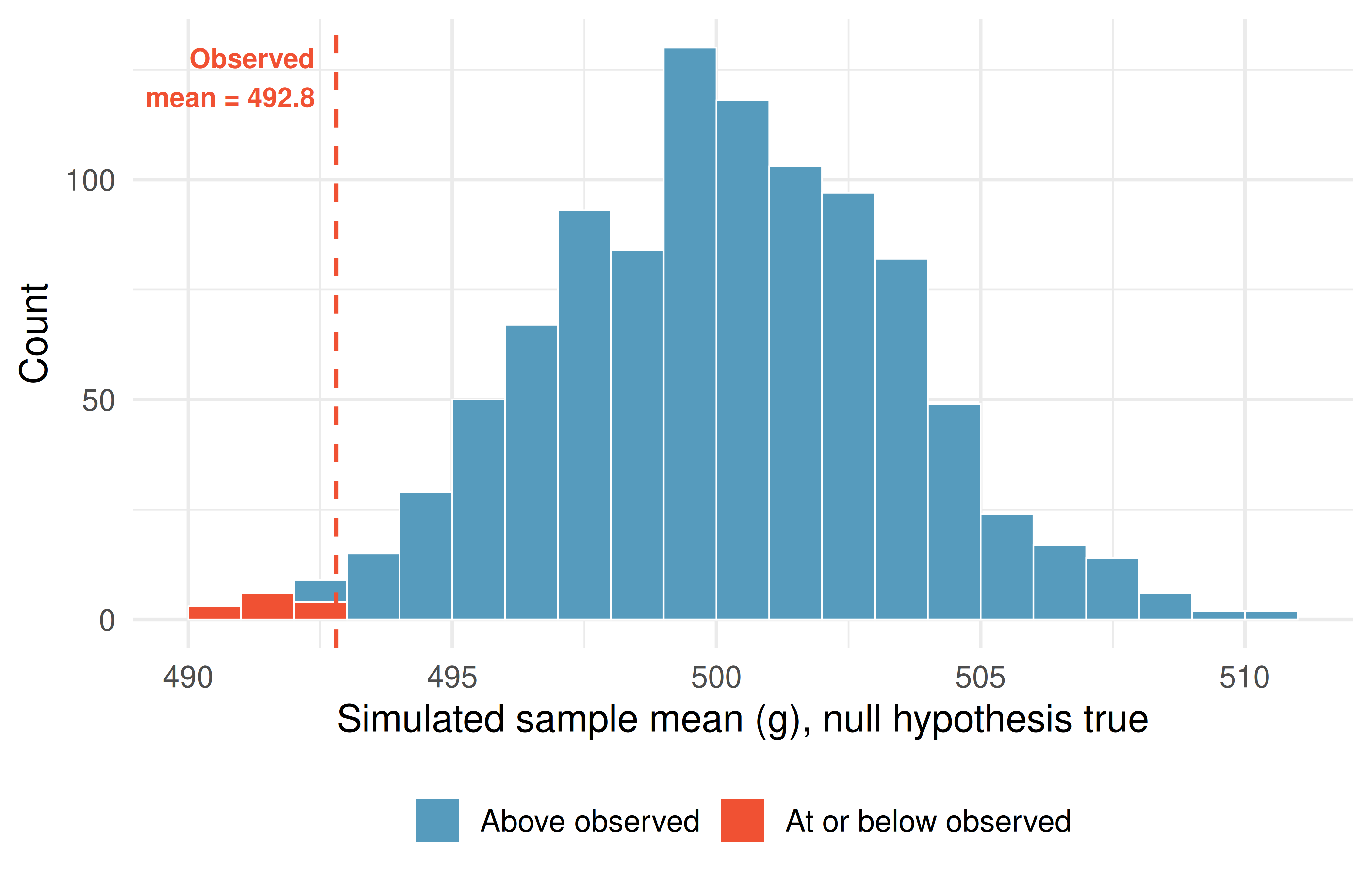
A bakery advertises that its sourdough loaves weigh 500 grams on average. A consumer group suspects the loaves are underfilled, weighs a random sample of 15 loaves, and finds a sample mean of 492.8 grams — about 7 grams light. Could a sample this light happen by chance when the true mean is 500 g?
We test \(H_0: \mu = 500\) against \(H_A: \mu < 500\). To simulate the null, we shift the 15 weights up so their mean is exactly 500, then repeatedly resample 15 loaves (with replacement) and record the mean of each.
The simulated means center on 500 g, as they must — we built the null world to make that true. The observed 492.8 g falls well into the left tail: a sample mean this low turns up only about 1% of the time when the true mean is really 500 g. That small \(p\)-value is evidence the loaves are underfilled.
Notice what this simulation assumed: only that the null is true and the sample is representative. No bell curve, no formula. The rest of this chapter develops the \(t\)-test — a mathematical shortcut that gives essentially the same answer when the data are roughly symmetric and the sample is not too small, and that comes with a formula you can compute by hand.
See it in action. Open the Randomization Test for a Single Mean to run this shift-and-resample test on your own data — enter a sample and a null value, generate the null distribution, and read the \(p\)-value off the tail.
14.2 The \(t\)-test framework
Every hypothesis test follows the same four-step structure — the same one we used for proportions — whether we use simulation or a mathematical model:
- State hypotheses. Write \(H_0\) (null hypothesis) and \(H_A\) (alternative hypothesis) in both words and symbols.
- Check conditions. Verify that the mathematical model is appropriate.
- Compute the test statistic and \(p\)-value. Calculate how far the observed data are from what \(H_0\) predicts, and determine how unusual that distance is.
- Draw a conclusion. Compare the \(p\)-value to the discernibility level \(\alpha\) and state the conclusion in context.
For means, the test statistic is a \(T\) score – the standardized distance from the observed sample mean to the hypothesized value, measured in units of standard errors.
See it in action. Guided walkthroughs for each \(t\)-test: one-sample · two-sample · paired. Each gates you through framing → conditions → test → interpretation. Or open the corresponding analytical CI + test tool directly on your own data.
14.3 One-sample \(t\)-test
14.3.1 Setup and hypotheses
The one-sample \(t\)-test is used when we have a single sample of quantitative data and want to test a claim about the population mean \(\mu\).
The test statistic for a single mean is a \(T\).
\[T = \frac{\bar{x} - \mu_0}{s / \sqrt{n}}\]
where \(\bar{x}\) is the sample mean, \(\mu_0\) is the hypothesized value from \(H_0\), \(s\) is the sample standard deviation, and \(n\) is the sample size.
When the null hypothesis is true and the conditions are met, \(T\) follows a \(t\)-distribution with \(df = n - 1\).
Conditions:
- Independent observations (e.g., random sample).
- Normality / sample size: The population distribution should be approximately normal, or \(n\) should be large enough (\(n \geq 30\)). Check for strong skewness or extreme outliers.
14.3.2 Worked example: Cherry Blossom race times
The average finishing time for all runners in the Cherry Blossom 10-mile race in 2006 was \(\mu = 93.29\) minutes. A random sample of 100 runners from a more recent year had a mean finishing time of \(\bar{x} = 97.32\) minutes with \(s = 16.98\) minutes. Is there evidence that the average finishing time has changed?
Step 1: State hypotheses.
- \(H_0\): \(\mu = 93.29\) (the average finishing time has not changed)
- \(H_A\): \(\mu \neq 93.29\) (the average finishing time has changed)
This is a two-sided test because we are looking for a change in either direction.
Step 2: Check conditions.
- Independence. The sample is a random sample of runners, so observations are independent.
- Sample size. With \(n = 100 \geq 30\), the CLT guarantees the sampling distribution of \(\bar{x}\) is approximately normal, even if the population distribution of finishing times is skewed.
Step 3: Compute the test statistic and \(p\)-value.
\[SE = \frac{s}{\sqrt{n}} = \frac{16.98}{\sqrt{100}} = 1.698\]
\[T = \frac{\bar{x} - \mu_0}{SE} = \frac{97.32 - 93.29}{1.698} = \frac{4.03}{1.698} = 2.37\]
With \(df = 100 - 1 = 99\), we find the area to the right of \(T = 2.37\) on the \(t\)-distribution: approximately 0.0099. Since this is a two-sided test, the \(p\)-value is \(2 \times 0.0099 = 0.0198\).
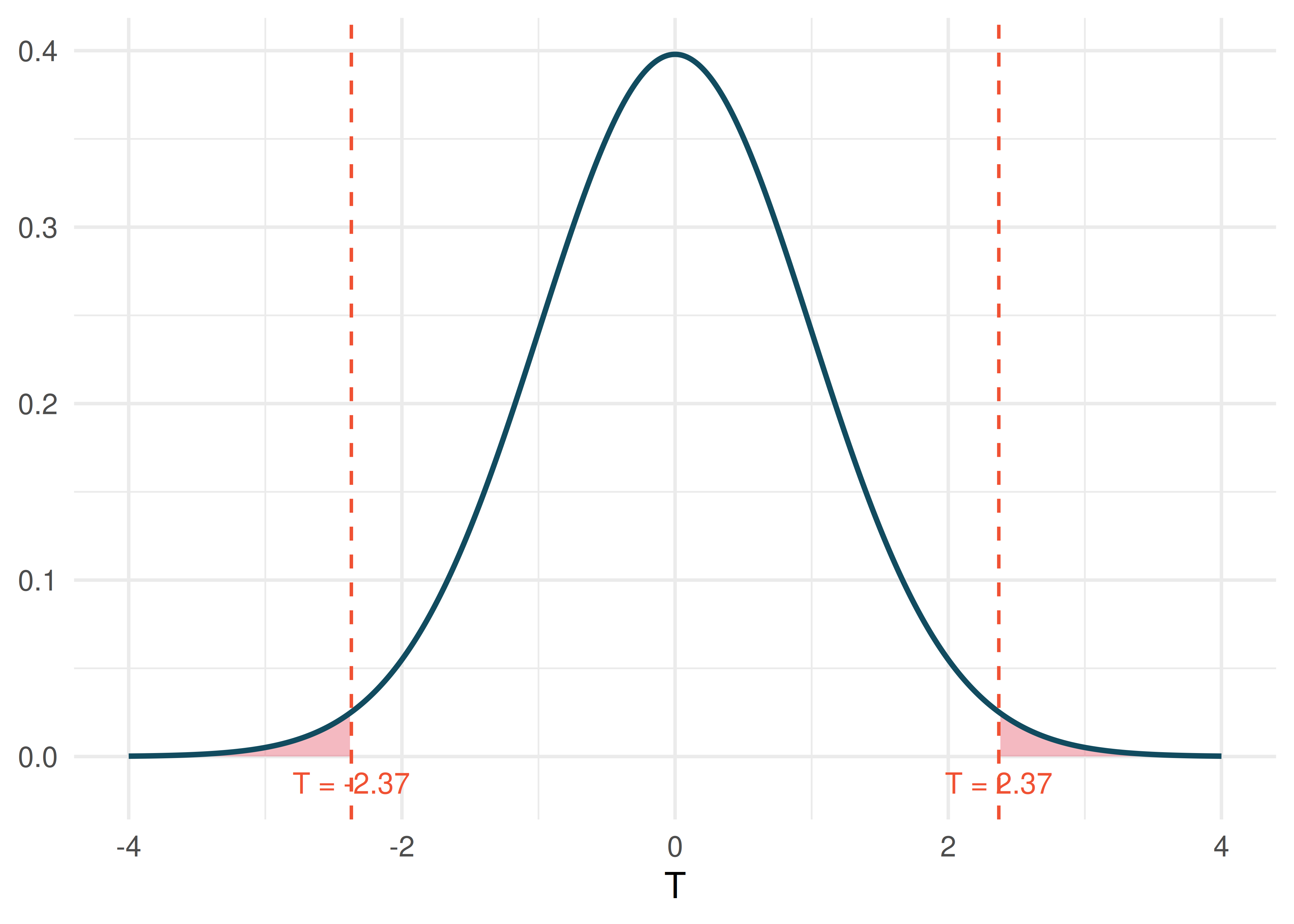
Step 4: Conclusion. The \(p\)-value of 0.0198 is less than \(\alpha = 0.05\), so we reject \(H_0\). The data provide statistically discernible evidence that the average finishing time has changed from the 2006 average of 93.29 minutes. Based on the sample, runners appear to be finishing more slowly on average.
A nutrition study claims that the average American adult consumes 2,000 mg of sodium per day. A random sample of 45 adults shows \(\bar{x} = 3,120\) mg and \(s = 1,100\) mg. Test whether the data provide evidence that the true average sodium intake differs from 2,000 mg. Use \(\alpha = 0.05\).
Show answer
Hypotheses: \(H_0: \mu = 2000\), \(H_A: \mu \neq 2000\). Conditions: random sample (independence), \(n = 45 \geq 30\) (normality via CLT). Test statistic: \(SE = 1100/\sqrt{45} = 163.9\), \(T = (3120 - 2000)/163.9 = 6.83\). With \(df = 44\), the two-tailed \(p\)-value is essentially 0 (far less than 0.05). We reject \(H_0\). There is very strong evidence that the average sodium intake is different from (and appears much higher than) 2,000 mg per day.14.4 Two-sample \(t\)-test
14.4.1 Setup and hypotheses
The two-sample \(t\)-test compares the means of two independent groups. The parameter of interest is \(\mu_1 - \mu_2\), and the null hypothesis typically claims no difference.
The test statistic for comparing two independent means is a \(T\).
\[T = \frac{(\bar{x}_1 - \bar{x}_2) - 0}{\sqrt{s_1^2/n_1 + s_2^2/n_2}}\]
When the null hypothesis is true and conditions are met, \(T\) follows a \(t\)-distribution with \(df = \min(n_1 - 1, n_2 - 1)\) (conservative approximation; software computes the exact \(df\)).
Conditions:
- Independence (extended). Observations are independent within and between the two groups.
- Normality / sample size. Each group should be approximately normal or have a large enough sample size. Check each group separately for strong skewness or extreme outliers.
14.4.2 Worked example: Birth weights and smoking
Is there evidence that newborns of mothers who smoke during pregnancy have a different average birth weight than newborns of non-smoking mothers? Data from a random sample of 1,000 US births in 2014:
| Group | \(n\) | Mean (lbs) | SD (lbs) |
|---|---|---|---|
| Nonsmoker | 867 | 7.27 | 1.23 |
| Smoker | 114 | 6.68 | 1.60 |
Step 1: State hypotheses.
- \(H_0\): \(\mu_n - \mu_s = 0\) (no difference in average birth weight)
- \(H_A\): \(\mu_n - \mu_s \neq 0\) (there is a difference in average birth weight)
Step 2: Check conditions.
- Independence. The data come from a simple random sample, so observations are independent within and between groups.
- Normality. Both groups have large sample sizes (\(n_n = 867\) and \(n_s = 114\)), both well above 30. Histograms of the data show no extreme outliers. Conditions are met.
Step 3: Compute the test statistic and \(p\)-value.
\[\bar{x}_n - \bar{x}_s = 7.27 - 6.68 = 0.59\]
\[SE = \sqrt{\frac{1.23^2}{867} + \frac{1.60^2}{114}} = \sqrt{\frac{1.5129}{867} + \frac{2.56}{114}} = \sqrt{0.001745 + 0.02246} = \sqrt{0.02420} = 0.156\]
\[T = \frac{0.59 - 0}{0.156} = 3.78\]
Using the conservative \(df = \min(867 - 1, 114 - 1) = 113\), the one-tail area for \(T = 3.78\) is approximately 0.000126. The two-tailed \(p\)-value is \(2 \times 0.000126 \approx 0.00025\).
Step 4: Conclusion. With a \(p\)-value of 0.00025, which is far less than \(\alpha = 0.05\), we reject \(H_0\). The data provide strong evidence that there is a difference in average birth weight between babies born to smoking and non-smoking mothers. Specifically, babies born to non-smoking mothers weigh about 0.59 lbs more on average.
14.4.3 Worked example: Exam versions
An instructor created two versions of an exam and randomly distributed them. Sample statistics:
| Version | \(n\) | Mean | SD | Min | Max |
|---|---|---|---|---|---|
| A | 58 | 75.1 | 13.9 | 44 | 100 |
| B | 55 | 72.0 | 13.8 | 38 | 100 |
Test whether there is convincing evidence that one version is more difficult. Use \(\alpha = 0.01\).
Step 1: State hypotheses.
- \(H_0\): \(\mu_A - \mu_B = 0\) (the exams are equally difficult)
- \(H_A\): \(\mu_A - \mu_B \neq 0\) (one exam is more difficult)
Step 2: Check conditions.
- Independence. Exams were randomly assigned, so independence is satisfied.
- Normality. Both groups have \(n > 30\) and the sample statistics suggest roughly symmetric distributions. Conditions are met.
Step 3: Compute the test statistic and \(p\)-value.
\[\bar{x}_A - \bar{x}_B = 75.1 - 72.0 = 3.1\]
\[SE = \sqrt{\frac{13.9^2}{58} + \frac{13.8^2}{55}} = \sqrt{\frac{193.21}{58} + \frac{190.44}{55}} = \sqrt{3.331 + 3.463} = \sqrt{6.794} = 2.607\]
\[T = \frac{3.1}{2.607} = 1.19\]
Using \(df = \min(57, 54) = 54\), the one-tail area for \(T = 1.19\) is about 0.12. The two-tailed \(p\)-value is approximately 0.24.
Step 4: Conclusion. The \(p\)-value of 0.24 is much larger than \(\alpha = 0.01\), so we fail to reject \(H_0\). The data do not provide convincing evidence that one exam version is more difficult than the other.
Does the conclusion above mean that the two exams are equally difficult?
Show answer
No. Failing to reject \(H_0\) does not prove that \(H_0\) is true. The data are consistent with the exams being equally difficult, but they are also consistent with exam A being about 3.1 points easier. The test simply did not find strong enough evidence to distinguish these possibilities.14.5 Paired \(t\)-test
14.5.1 Setup and hypotheses
When data are paired (see the confidence intervals for means chapter for what makes data “paired”), we compute the difference within each pair and test whether the mean difference is zero.
The test statistic for a paired mean difference is a \(T\).
\[T = \frac{\bar{x}_{diff} - 0}{s_{diff} / \sqrt{n_{diff}}}\]
When the null hypothesis is true and conditions are met, \(T\) follows a \(t\)-distribution with \(df = n_{diff} - 1\).
Conditions:
- Independently sampled pairs.
- Normality of differences. The differences should be approximately normal, or \(n_{diff}\) should be large. Check for extreme outliers in the differences.
Optional — see it by simulation. The paired test can also be run by simulation, as in the randomization tests chapter. Because the null says there is no difference, the two measurements in each pair are interchangeable, so we flip the sign of each difference at random, recompute the mean, and repeat to build a null distribution centered at zero. Open the Paired Randomization Test to try it. (Because it keeps the magnitudes of the differences, this is the sign-flip randomization test — not the lower-power nonparametric sign test, which counts only the signs.)
14.5.2 Worked example: Textbook prices
Is there evidence that UCLA Bookstore prices differ from Amazon prices, on average? Sample statistics for the 68 price differences (UCLA \(-\) Amazon):
| \(n_{diff}\) | \(\bar{x}_{diff}\) | \(s_{diff}\) |
|---|---|---|
| 68 | $3.58 | $13.42 |
Step 1: State hypotheses.
- \(H_0\): \(\mu_{diff} = 0\) (no difference in average textbook price)
- \(H_A\): \(\mu_{diff} \neq 0\) (there is a difference in average price)
Step 2: Check conditions.
- Independence. The textbooks were a simple random sample of courses; pairs are independent.
- Normality. With \(n_{diff} = 68\), the CLT applies. While some outliers exist (a few textbooks with large price differences), none are extreme enough to invalidate the approach given the large sample size.
Step 3: Compute the test statistic and \(p\)-value.
\[SE = \frac{s_{diff}}{\sqrt{n_{diff}}} = \frac{13.42}{\sqrt{68}} = 1.628\]
\[T = \frac{3.58 - 0}{1.628} = 2.20\]
With \(df = 68 - 1 = 67\), the one-tail area for \(T = 2.20\) is approximately 0.0156. The two-tailed \(p\)-value is \(2 \times 0.0156 = 0.0312\).
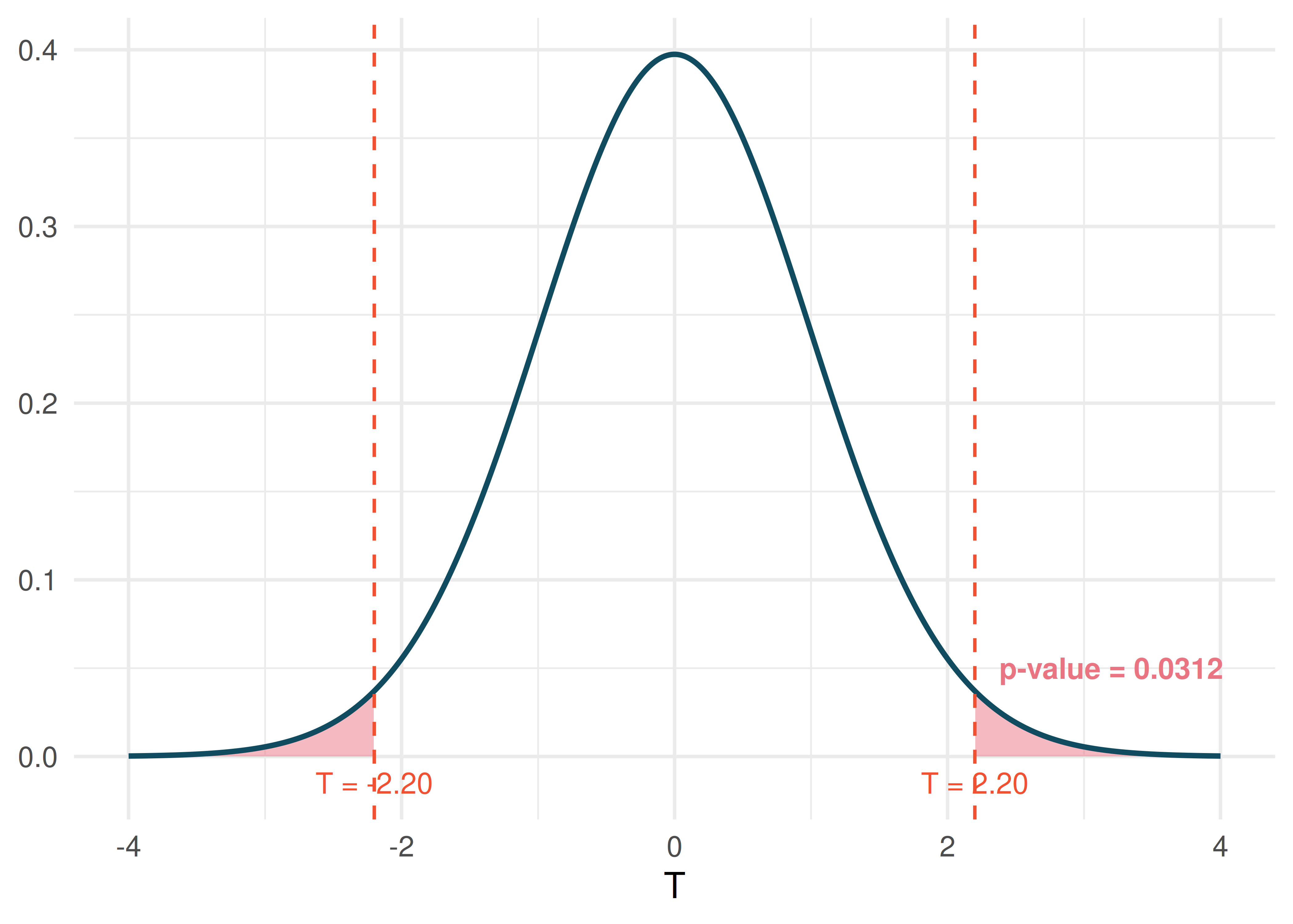
Step 4: Conclusion. The \(p\)-value of 0.0312 is less than \(\alpha = 0.05\), so we reject \(H_0\). The data provide evidence that UCLA Bookstore prices are different from Amazon prices on average. Based on the positive mean difference, the UCLA Bookstore tends to charge more.
Researchers measured tire tread (in cm) for 25 cars, each equipped with one Smooth Turn and one Quick Spin tire. The mean tread difference (Smooth Turn \(-\) Quick Spin) was \(\bar{x}_{diff} = 0.002\) cm with \(s_{diff} = 0.004\) cm. Test whether there is a difference in average tread wear between the two brands. Use \(\alpha = 0.05\).
Show answer
Hypotheses: \(H_0: \mu_{diff} = 0\), \(H_A: \mu_{diff} \neq 0\). Conditions: cars are independent, \(n = 25\) and no extreme outliers reported. \(SE = 0.004/\sqrt{25} = 0.0008\). \(T = 0.002/0.0008 = 2.50\). With \(df = 24\), the two-tailed \(p\)-value is approximately 0.020. Since \(0.020 < 0.05\), we reject \(H_0\) and conclude there is evidence of a difference in tread wear between the two tire brands.14.6 Connecting simulation-based and \(t\)-based tests
An important theme throughout this course is that simulation-based methods and mathematical models are complementary approaches to the same questions. When conditions are met, they should give similar answers. Here we compare the two approaches explicitly.
14.6.1 When they agree
For the birth weights example:
- Randomization test: Shuffle smoking/nonsmoking labels 10,000 times, compute the difference in means each time, and find the proportion of shuffled differences as extreme as 0.59 lbs. A difference that large essentially never appears (typically 0 of the 10,000 shuffles), so the \(p\)-value is below 0.0001.
- \(t\)-test: The \(p\)-value was 0.00025.
Both approaches lead to the same conclusion (reject \(H_0\)) by a wide margin. This agreement is typical when sample sizes are moderate to large and conditions are met.
14.6.2 When they might disagree
Disagreement arises primarily in two situations:
- Small samples from skewed populations. The \(t\)-test assumes the sampling distribution is symmetric, which may not hold for small samples from skewed distributions. A simulation-based approach can capture the asymmetry.
- Extreme outliers. The \(t\)-test relies on \(\bar{x}\) and \(s\), both of which are sensitive to outliers. A randomization test builds its null distribution by shuffling the actual data instead of assuming a \(t\) model, so its \(p\)-value does not depend on the normality assumption that outliers undermine (although the difference in means itself is still pulled around by outliers).
14.6.3 Practical guidance
- When conditions are clearly met (large samples, no extreme outliers), use the \(t\)-test – it is simpler and faster.
- When conditions are borderline (moderate samples, mild skewness), consider running both approaches. If they agree, report the \(t\)-test. If they disagree, investigate why and consider the simulation-based result more trustworthy.
- When conditions are clearly violated (small samples, strong skewness, extreme outliers), prefer the simulation-based approach.
14.7 Practical vs. statistical discernibility
Statistical discernibility \(\neq\) practical importance.
A result is statistically discernible if the \(p\)-value is below the chosen discernibility level \(\alpha\). But statistical discernibility only means the observed effect is unlikely to be due to chance alone. It says nothing about whether the effect is large enough to matter in practice.
With very large samples, even trivially small differences can be statistically discernible. With very small samples, even large differences may not be statistically discernible (due to low power).
A large study of 50,000 students found that students who eat breakfast score an average of 0.5 points higher on a 100-point exam than students who skip breakfast (\(p < 0.001\)). Is this result practically important?
The result is statistically discernible (the \(p\)-value is very small), but the effect size of 0.5 points on a 100-point exam is tiny. A teacher or student would likely not consider half a point to be a meaningful difference. This is an example where statistical discernibility does not imply practical importance.
14.7.1 Effect sizes
To bridge the gap between statistical and practical importance, researchers often report effect sizes – standardized measures of how large the observed effect is.
Cohen’s \(d\) is a common measure of effect size for comparing two means. It expresses the difference in means as a multiple of the pooled standard deviation:
\[d = \frac{\bar{x}_1 - \bar{x}_2}{s_p}\]
where \(s_p\) is the pooled standard deviation. General guidelines for interpreting \(d\):
| \(|d|\) | Interpretation |
|---|---|
| 0.2 | Small effect |
| 0.5 | Medium effect |
| 0.8 | Large effect |
These guidelines are rough benchmarks. What constitutes a “meaningful” effect depends on the context. In medicine, even a small effect size might be important if it concerns a life-threatening condition. In education, a medium effect might be required for a costly intervention to be worthwhile.
In the birth weights study, the difference was 0.59 lbs with a pooled standard deviation of approximately 1.28 lbs. Compute Cohen’s \(d\) and interpret it.
Show answer
\(d = 0.59 / 1.28 = 0.46\). This is between a small and medium effect. While the difference is statistically discernible, the practical impact is moderate – about half a standard deviation in birth weight.14.8 Chapter review
14.8.1 Summary
This chapter presented hypothesis tests for means using the \(t\)-distribution:
- One-sample \(t\)-test: Tests whether a population mean \(\mu\) equals a hypothesized value \(\mu_0\). Test statistic: \(T = \frac{\bar{x} - \mu_0}{s/\sqrt{n}}\) with \(df = n - 1\).
- Two-sample \(t\)-test: Tests whether two population means are equal. Test statistic: \(T = \frac{(\bar{x}_1 - \bar{x}_2)}{\sqrt{s_1^2/n_1 + s_2^2/n_2}}\) with \(df = \min(n_1 - 1, n_2 - 1)\).
- Paired \(t\)-test: Tests whether the mean of paired differences equals zero. Compute differences first, then apply the one-sample \(t\)-test to the differences: \(T = \frac{\bar{x}_{diff}}{s_{diff}/\sqrt{n_{diff}}}\) with \(df = n_{diff} - 1\).
- All three tests require independence and approximate normality or large sample size.
- Simulation-based and \(t\)-based tests generally agree when conditions are met. When conditions are questionable, simulation is more reliable.
- Statistical discernibility (small \(p\)-value) does not imply practical importance (large enough to matter). Effect sizes like Cohen’s \(d\) help assess practical importance.
14.8.2 Key terms
\(T\) test statistic, one-sample \(t\)-test, two-sample \(t\)-test, paired \(t\)-test, degrees of freedom, \(p\)-value, discernibility level (\(\alpha\)), statistical discernibility, practical importance, effect size, Cohen’s \(d\).
14.9 Exercises
Answers to odd-numbered exercises are provided in the Exercise Solutions appendix at the back of the book.
- Find the p-value, I. A random sample is selected from an approximately normal population with an unknown standard deviation. Find the p-value for the given sample size and test statistic. Also determine if the null hypothesis would be rejected at \(\alpha = 0.05\).
\(n = 11\), \(T = 1.91\)
\(n = 17\), \(T = -3.45\)
\(n = 7\), \(T = 0.83\)
\(n = 28\), \(T = 2.13\)
- Find the p-value, II. A random sample is selected from an approximately normal population with an unknown standard deviation. Find the p-value for the given sample size and test statistic. Also determine if the null hypothesis would be rejected at \(\alpha = 0.01\).
\(n = 26\), \(T = 2.485\)
\(n = 18\), \(T = 0.5\)
- Length of gestation, hypothesis test. In this exercise we work with a random sample of 1,000 cases from the dataset released by the United States Department of Health and Human Services in 2014. Provided below are sample statistics for gestation (length of pregnancy, measured in weeks) of births in this sample.
| Min | Q1 | Median | Mean | Q3 | Max | SD | IQR |
|---|---|---|---|---|---|---|---|
| 21 | 38 | 39 | 38.7 | 40 | 46 | 2.6 | 2 |
What is the point estimate for the average length of pregnancy for all women? What about the median?
You might have heard that human gestation is typically 40 weeks. Using the data, perform a complete hypothesis test, using mathematical models, to assess the 40 week claim. State the null and alternative hypotheses, find the T score, find the p-value, and provide a conclusion in context of the data.
A quick internet search validates the claim of “40 weeks gestation” for humans. A friend of yours claims that there are different ways to measure gestation (starting at first day of last period, ovulation, or conception) which will result in estimates that are a week or two different. Another friend mentions that recent increases in cesarean births is likely to have decreased length of gestation. Do the data provide a mechanism to distinguish between your two friends’ claims?
- Interpreting p-values for population mean. For each of the following statements, indicate if they are a true or false interpretation of the p-value. If false, provide a reason or correction to the misinterpretation. You are wondering if the average amount of cereal in a 10oz cereal box is greater than 10oz. You collect 50 boxes of cereal, weigh them carefully, find a T score, and a p-value of 0.23.
The probability that the average weight of all cereal boxes is 10 oz is 0.23.
The probability that the average weight of all cereal boxes is greater than 10 oz is 0.23.
Because the p-value is 0.23, the average weight of all cereal boxes is 10 oz.
Because the p-value is small, the population average must be just barely above 10 oz.
If \(H_0\) is true, the probability of observing another sample with an average as or more extreme as the data is 0.23.
- Sleep habits of New Yorkers. New York is known as “the city that never sleeps”. A random sample of 25 New Yorkers were asked how much sleep they get per night. Statistical summaries of these data are shown below. The point estimate suggests New Yorkers sleep less than 8 hours a night on average. Evaluate the claim that New York is the city that never sleeps keeping in mind that, despite this claim, the true average number of hours New Yorkers sleep could be less than 8 hours or more than 8 hours.
| n | Mean | SD | Min | Max |
|---|---|---|---|---|
| 25 | 7.73 | 0.77 | 6.17 | 9.78 |
Write the hypotheses in symbols and in words.
Check conditions, then calculate the test statistic, \(T\), and the associated degrees of freedom.
Find and interpret the p-value in this context. Drawing a picture may be helpful.
What is the conclusion of the hypothesis test?
If you were to construct a 90% confidence interval that corresponded to this hypothesis test, would you expect 8 hours to be in the interval?
- Find the mean. You are given the hypotheses shown below. We know that the sample standard deviation is 8 and the sample size is 20. For what sample mean would the p-value be equal to 0.05? Assume that all conditions necessary for inference are satisfied.
\[H_0: \mu = 60 \quad \quad H_A: \mu \neq 60\]
- Play the piano. Georgianna claims that in a small city renowned for its music school, the average child takes less than 5 years of piano lessons. We have a random sample of 20 children from the city, with a mean of 4.6 years of piano lessons and a standard deviation of 2.2 years.
Evaluate Georgianna’s claim (or that the opposite might be true) using a hypothesis test.
Construct a 95% confidence interval for the number of years students in this city take piano lessons, and interpret it in context of the data.
Do your results from the hypothesis test and the confidence interval agree? Explain your reasoning.
- Auto exhaust and lead exposure. Researchers interested in lead exposure due to car exhaust sampled the blood of 52 police officers subjected to constant inhalation of automobile exhaust fumes while working traffic enforcement in a primarily urban environment. The blood samples of these officers had an average lead concentration of 124.32 \(\mu\)g/l and a SD of 37.74 \(\mu\)g/l; a previous study of individuals from a nearby suburb, with no history of exposure, found an average blood level concentration of 35 \(\mu\)g/l. (Mortada et al. 2000)
Write down the hypotheses that would be appropriate for testing if the police officers appear to have been exposed to a different concentration of lead.
Explicitly state and check all conditions necessary for inference on these data.
Test the hypothesis that the downtown police officers have a higher lead exposure than the group in the previous study. Interpret your results in context.
- Experimental baker. A baker working on perfecting their bagel recipe is experimenting with active dry (AD) and instant (I) yeast. They bake a dozen bagels with each type of yeast and score each bagel on a scale of 1 to 10 on how well the bagels rise. They come up with the following set of hypotheses for evaluating whether there is a difference in the average rise of bagels baked with active dry and instant yeast. What is wrong with the hypotheses as stated?
\[H_0: \bar{x}_{AD} \leq \bar{x}_{I} \quad \quad H_A: \bar{x}_{AD} > \bar{x}_{I}\]
- Diamonds, randomization test. The prices of diamonds go up as the carat weight increases, but the increase is not smooth. For example, the difference between the size of a 0.99 carat diamond and a 1 carat diamond is undetectable to the naked human eye, but the price of a 1 carat diamond tends to be much higher than the price of a 0.99 carat diamond. We have two random samples of diamonds: 23 0.99 carat diamonds and 23 1 carat diamonds. In order to be able to compare equivalent units, we first divide the price for each diamond by 100 times its weight in carats. That is, for a 0.99 carat diamond, we divide the price by 99 and for a 1 carat diamond, we divide it by 100. Then, we randomize the carat weight to the price values in order simulate the null distribution of differences in average prices of 0.99 carat and 1 carat diamonds. The null distribution (with 1,000 randomized differences) is shown below and depicts the distribution of differences in sample means (of price per carat) if there really was no difference in the population from which these diamonds came. (Wickham 2016)
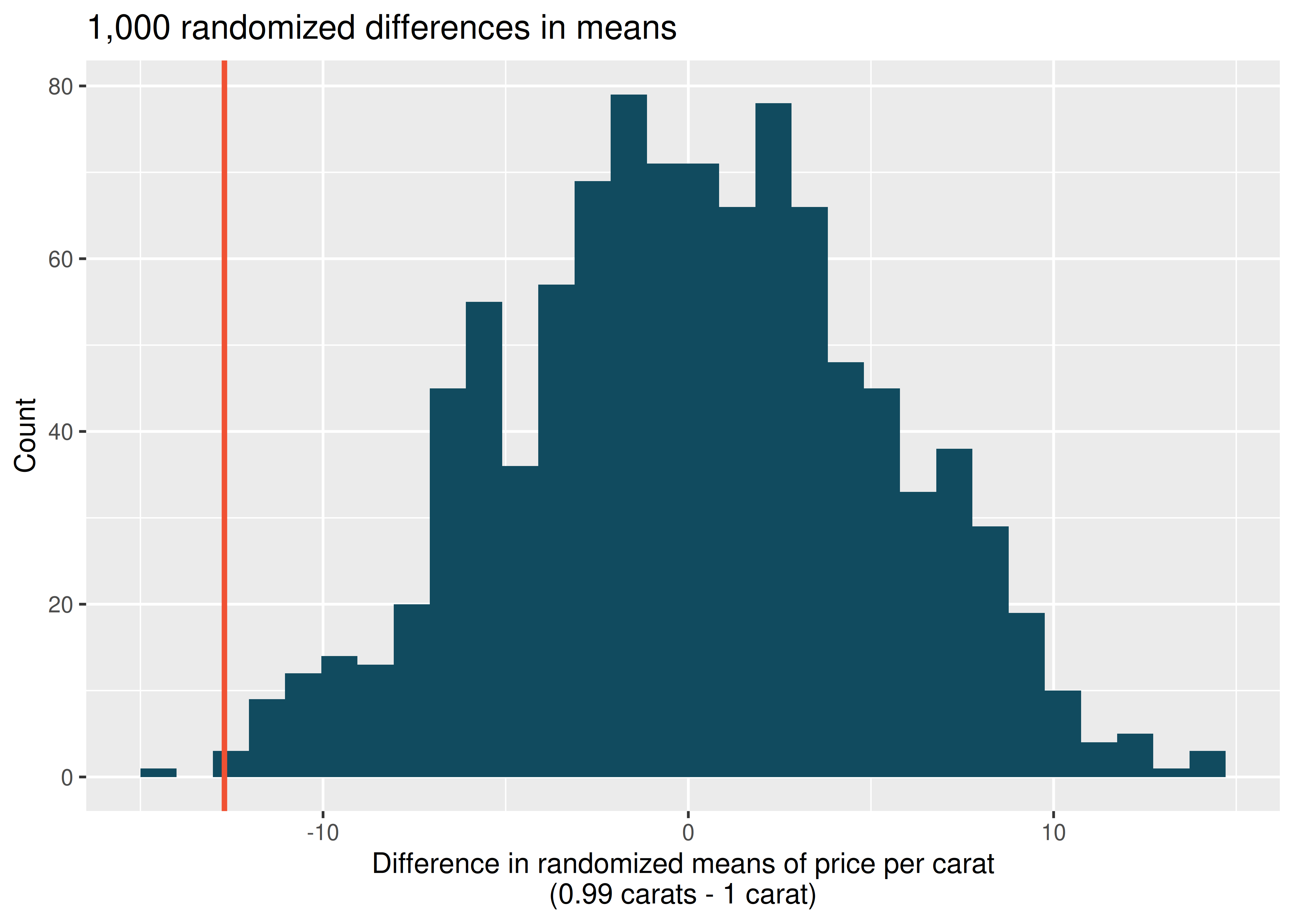
Using the randomization distribution, conduct a hypothesis test to evaluate if there is a difference between the prices per carat of diamonds that weigh 0.99 carats and diamonds that weigh 1 carat. Make sure to state your hypotheses clearly and interpret your results in context of the data. (Wickham 2016)
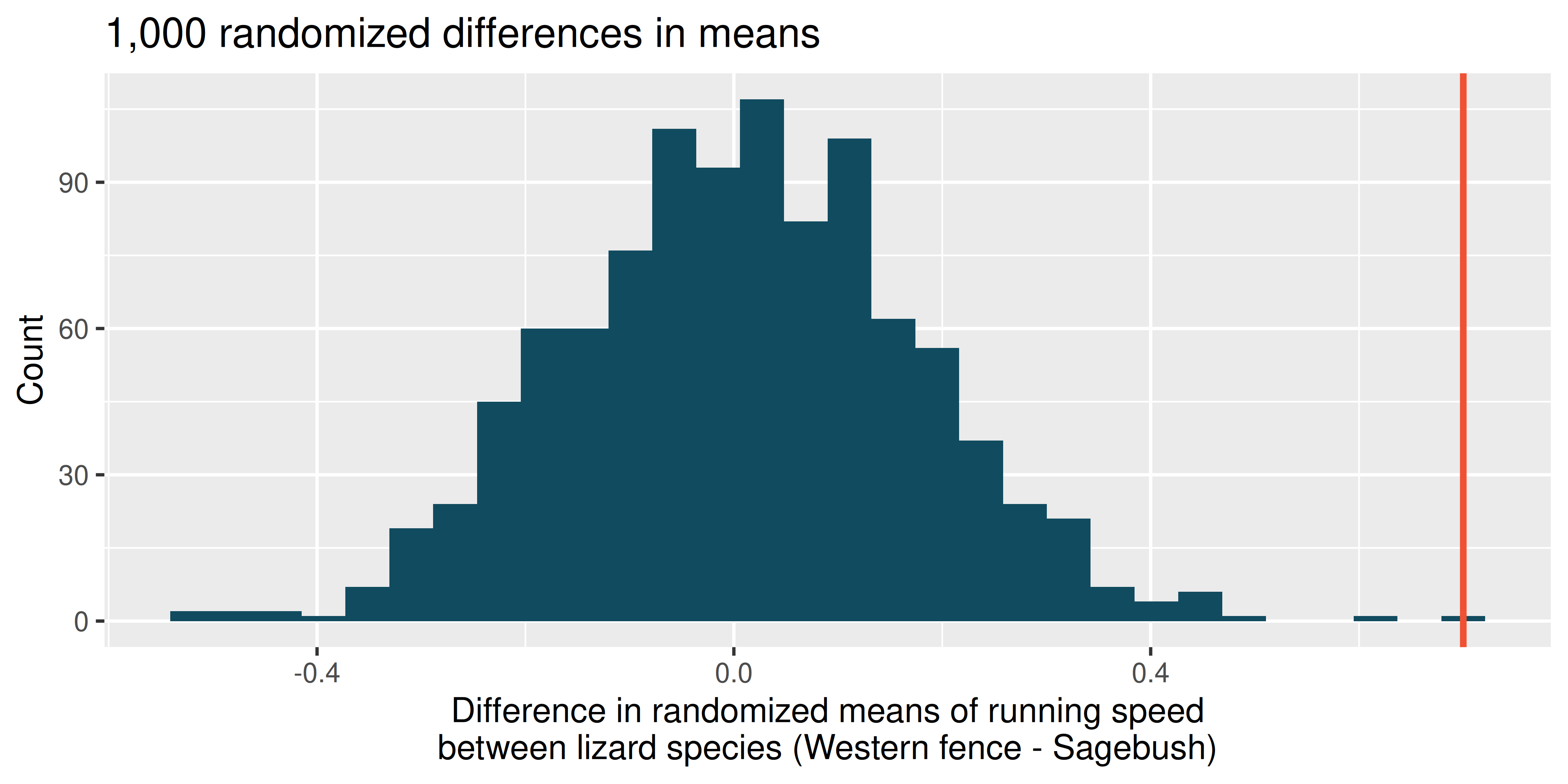
- Lizards running, randomization test. In order to assess physiological characteristics of common lizards, data on top speeds (in m/sec) measured on a laboratory race track for two species of lizards: Western fence lizard (Sceloporus occidentalis) and Sagebrush lizard (Sceloporus graciosus). The original observed difference in lizard speeds is \(\bar{x}_{Western fence} - \bar{x}_{Sagebrush} = 0.7 \mbox{m/sec}.\) The histogram below shows the distribution of average differences when speed has been randomly allocated across lizard species 1,000 times. Using the randomization distribution, conduct a hypothesis test to evaluate if there is a difference between the average speed of the Western fence lizard as compared to the Sagebrush lizard. Make sure to state your hypotheses clearly and interpret your results in context of the data. (Adolph 1987)
- Possible randomized means. Data were collected on data from two groups (A and B). There were 3 measurements taken on Group A and two measurements in Group B.
| Group | Measurement 1 | Measurement 2 | Measurement 3 |
|---|---|---|---|
| A | 1 | 15 | 5 |
| B | 7 | 3 | NA |
If the data are (repeatedly) randomly allocated across the two conditions, provide the following: (1) the values which are assigned to group A, (2) the values which are assigned to group B, and (3) the difference in averages \((\bar{x}_A - \bar{x}_B)\) for each of the following:
When the randomized difference in averages is as large as possible.
When the randomized difference in averages is as small as possible (a big in magnitude negative number).
When the randomized difference in averages is as close to zero as possible.
When the observed values are randomly assigned to the two groups, to which of the previous parts would you expect the difference in means to fall closest? Explain your reasoning.
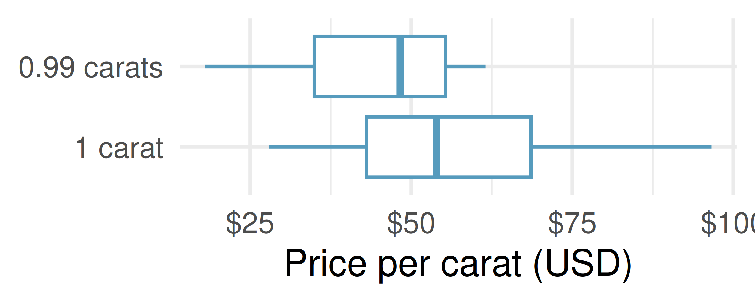
- Diamonds, mathematical test. We have data on two random samples of diamonds: one with diamonds that weigh 0.99 carats and one with diamonds that weigh 1 carat. Each sample has 23 diamonds. Sample statistics for the price per carat of diamonds in each sample are provided below. Conduct a hypothesis test using a mathematical model to evaluate if there is a difference between the prices per carat of diamonds that weigh 0.99 carats and diamonds that weigh 1 carat Make sure to state your hypotheses clearly, check relevant conditions, and interpret your results in context of the data. (Wickham 2016)
| Mean | SD | n | |
|---|---|---|---|
| 0.99 carats | $44.51 | $13.32 | 23 |
| 1 carat | $57.20 | $18.19 | 23 |
- A/B testing. A/B testing is a user experience research methodology where two variants of a page are shown to users at random. A company wants to evaluate whether users will spend more time, on average, on Page A or Page B using an A/B test. Two user experience designers at the company, Lucie and Müge, are tasked with conducting the analysis of the data collected. They agree on how the null hypothesis should be set: on average, users spend the same amount of time on Page A and Page B. Lucie believes that Page B will provide a better experience for users and hence wants to use a one-tailed test, Müge believes that a two-tailed test would be a better choice. Which designer do you agree with, and why?
- Mindfulness intervention for nurses. In order to address extremely challenging and stressful situations for intensive care unit nurses, researchers ran a mindfulness-based intervention (MBI) study on 60 nurses working in three hospitals in El-Beheira, Egypt. The participants were randomly allocated to one of the two groups: the treatment group (MBI) received 8 MBI sessions and the control group received no intervention. The nurses’ emotional exhaustion was measured using 9 items from a questionnaire of the Maslach Burnout Inventory-Human Services Survey for Medical Personnel; the questions are recorded on a Likert scale where 0 indicated “Never” and 6 indicates “Every day”. Nurses in the treatment group had an emotional exhaustion score of 15.47, with a standard deviation of 4.44, and nurses in the control group had an emotional exhaustion score of 32.43, with a standard deviation of 8.87. Do these data provide convincing evidence that the emotional exhaustion decrease is different for the patients in the treatment group compared to the control group? Assume that conditions for conducting inference using mathematical models are satisfied. (Othman, Hassan, and Mohamed 2023)
- Chicken diet: horsebean vs. linseed. Chicken farming is a multi-billion dollar industry, and any methods that increase the growth rate of young chicks can reduce consumer costs while increasing company profits, possibly by millions of dollars. An experiment was conducted to measure and compare the effectiveness of various feed supplements on the growth rate of chickens. Newly hatched chicks were randomly allocated into six groups, and each group was given a different feed supplement. In this exercise we consider chicks that were fed horsebean and linseed. Below are some summary statistics from this dataset along with box plots showing the distribution of weights by feed type. (McNeil 1977)
| Horsebean | Linseed | |
|---|---|---|
| Mean | 160.2 | 218.8 |
| SD | 38.6 | 52.2 |
| n | 10.0 | 12.0 |
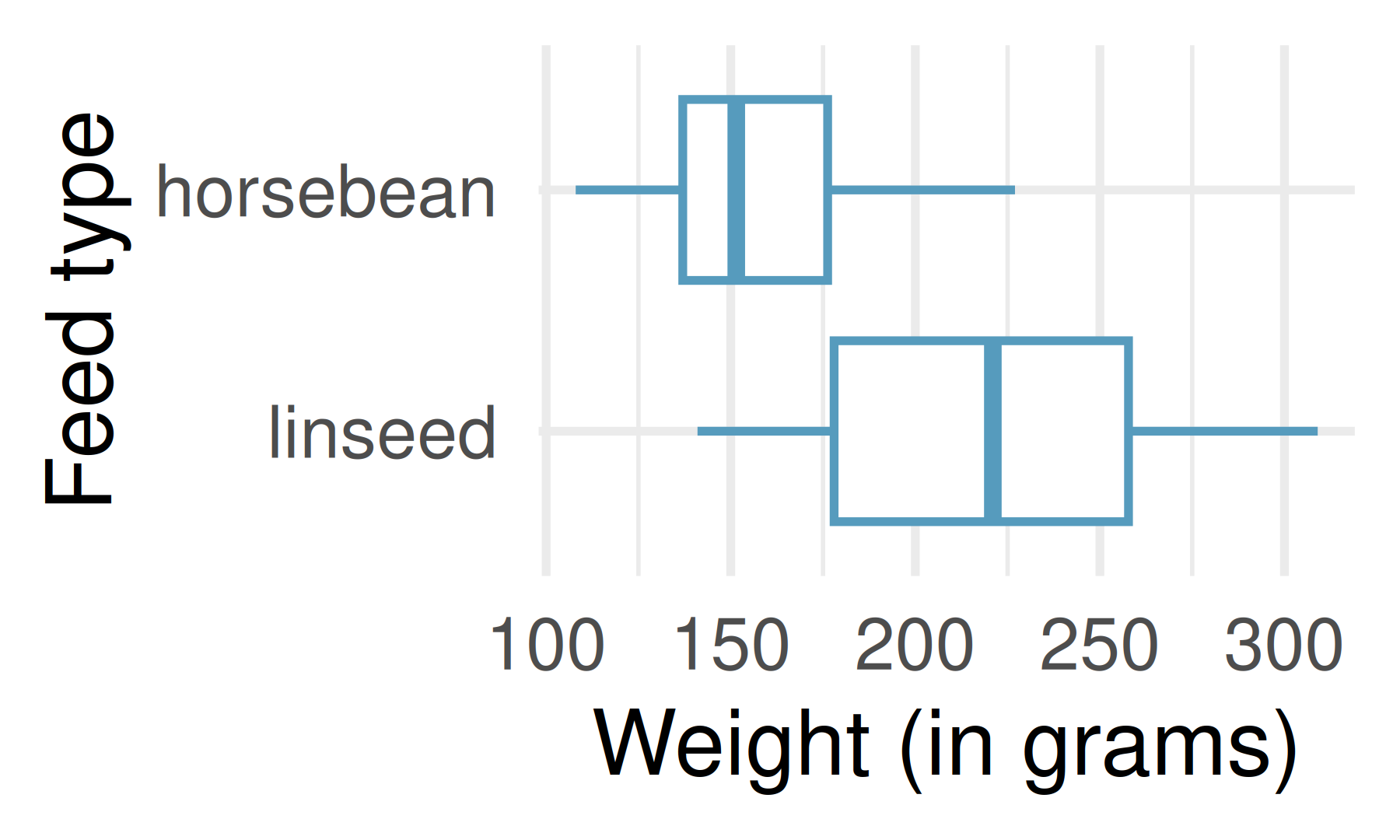
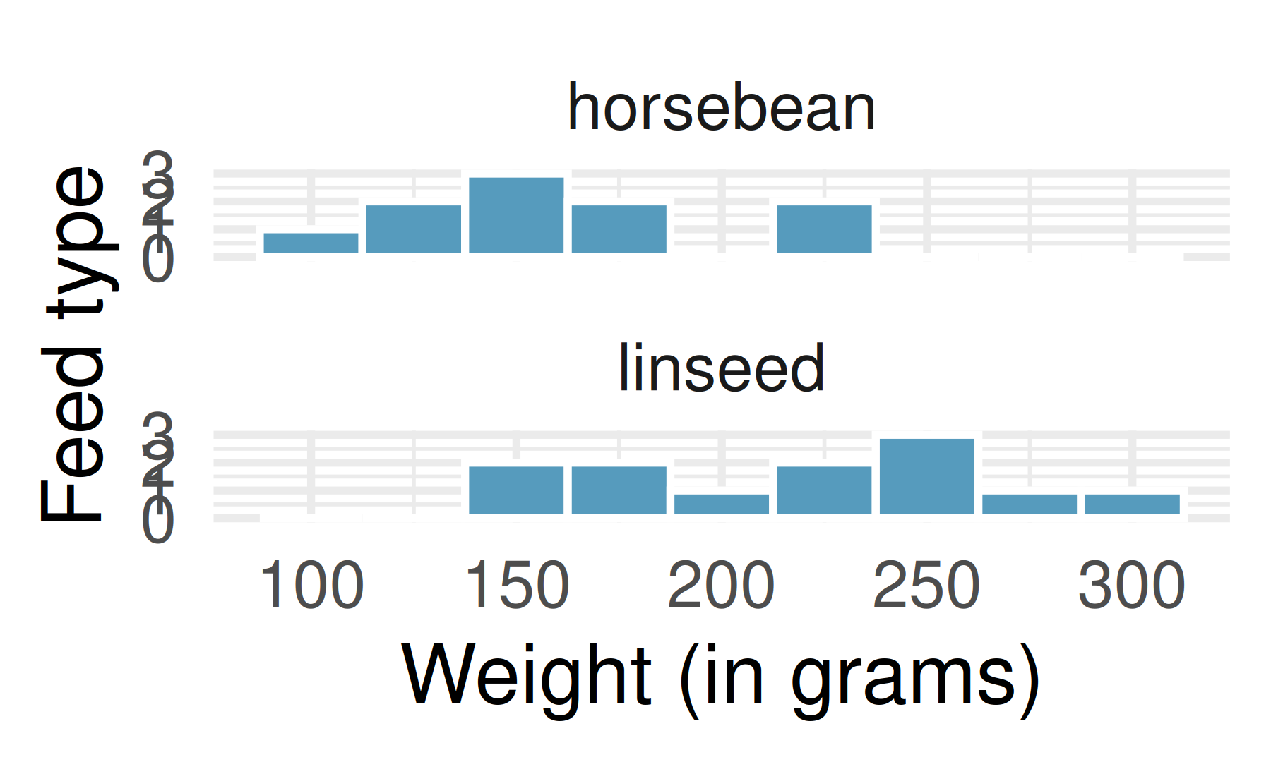
Describe the distributions of weights of chickens that were fed horsebean and linseed.
Do these data provide strong evidence that the average weights of chickens that were fed linseed and horsebean are different? Use a 5% discernibility level.
What type of error might we have committed? Explain.
Would your conclusion change if we used \(\alpha = 0.01\)?
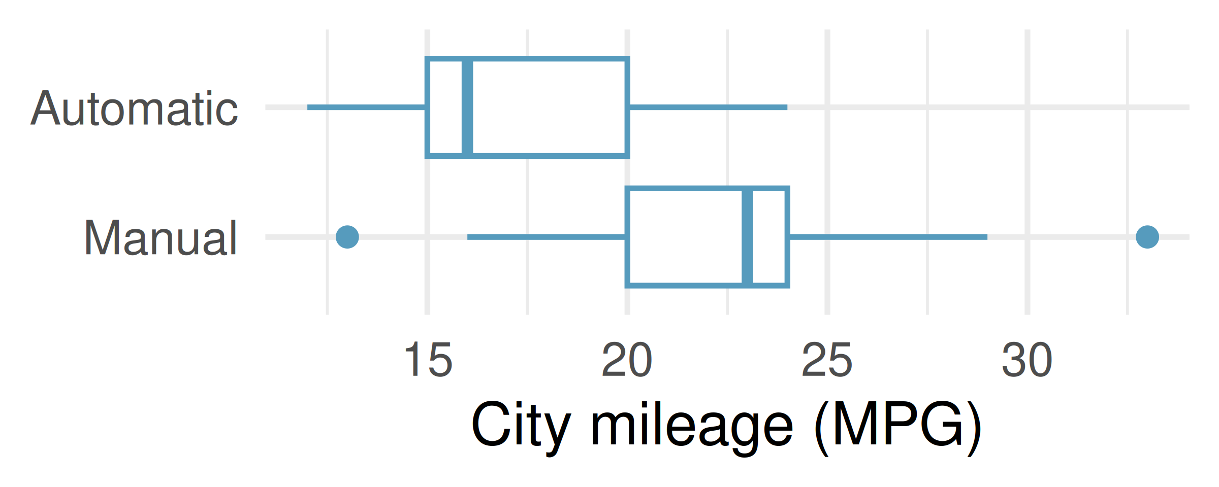
- Fuel efficiency in the city. Each year the US Environmental Protection Agency (EPA) releases fuel economy data on cars manufactured in that year. Below are summary statistics on fuel efficiency (in miles/gallon) from random samples of cars with manual and automatic transmissions manufactured in 2021. Do these data provide strong evidence of a difference between the average fuel efficiency of cars with manual and automatic transmissions in terms of their average city mileage? (US DOE EPA 2021)
| CITY | Mean | SD | n |
|---|---|---|---|
| Automatic | 17.4 | 3.44 | 25 |
| Manual | 22.7 | 4.58 | 25 |
- Chicken diet: casein vs. soybean. Casein is a common weight gain supplement for humans. Does it have an effect on chickens? An experiment was conducted to measure and compare the effectiveness of various feed supplements on the growth rate of chickens. Newly hatched chicks were randomly allocated into six groups, and each group was given a different feed supplement. In this exercise we consider chicks that were fed casein and soybean. Assume that the conditions for conducting inference using mathematical models are met, and using the data provided below, test the hypothesis that the average weight of chickens that were fed casein is different than the average weight of chickens that were fed soybean. If your hypothesis test yields a statistically discernible result, discuss whether the higher average weight of chickens can be attributed to the casein diet. (McNeil 1977)
| Feed type | Mean | SD | n |
|---|---|---|---|
| casein | 323.58 | 64.43 | 12 |
| soybean | 246.43 | 54.13 | 14 |
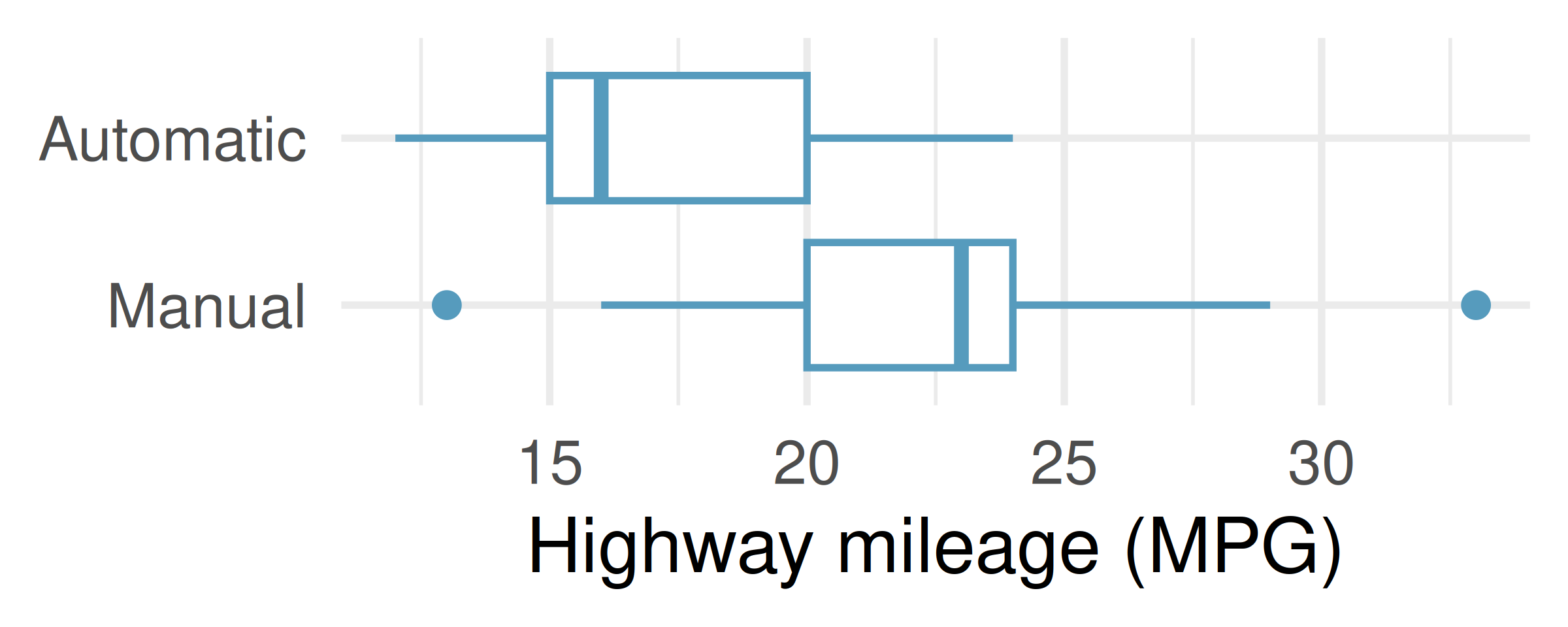
- Fuel efficiency on the highway. Each year the US Environmental Protection Agency (EPA) releases fuel economy data on cars manufactured in that year. Below are summary statistics on fuel efficiency (in miles/gallon) from random samples of cars with manual and automatic transmissions manufactured in 2021. Do these data provide strong evidence of a difference between the average fuel efficiency of cars with manual and automatic transmissions in terms of their average highway mileage? (US DOE EPA 2021)
| HIGHWAY | Mean | SD | n |
|---|---|---|---|
| Automatic | 23.7 | 3.90 | 25 |
| Manual | 30.9 | 5.13 | 25 |
- Gaming, distracted eating, and intake. A group of researchers who are interested in the possible effects of distracting stimuli during eating, such as an increase or decrease in the amount of food consumption, monitored food intake for a group of 44 patients who were randomized into two equal groups. The treatment group ate lunch while playing solitaire, and the control group ate lunch without any added distractions. Patients in the treatment group ate 52.1 grams of biscuits, with a standard deviation of 45.1 grams, and patients in the control group ate 27.1 grams of biscuits, with a standard deviation of 26.4 grams. Do these data provide convincing evidence that the average food intake (measured in amount of biscuits consumed) is different for the patients in the treatment group compared to the control group? Assume that conditions for conducting inference using mathematical models are satisfied. (Oldham-Cooper et al. 2011)
- Gaming, distracted eating, and recall. A group of researchers who are interested in the possible effects of distracting stimuli during eating, such as an increase or decrease in the amount of food consumption, monitored food intake for a group of 44 patients who were randomized into two equal groups. The 22 patients in the treatment group who ate their lunch while playing solitaire were asked to do a serial-order recall of the food lunch items they ate. The average number of items recalled by the patients in this group was 4. 9, with a standard deviation of 1.8. The average number of items recalled by the patients in the control group (no distraction) was 6.1, with a standard deviation of 1.8. Do these data provide strong evidence that the average numbers of food items recalled by the patients in the treatment and control groups are different? Assume that conditions for conducting inference using mathematical models are satisfied. (Oldham-Cooper et al. 2011)
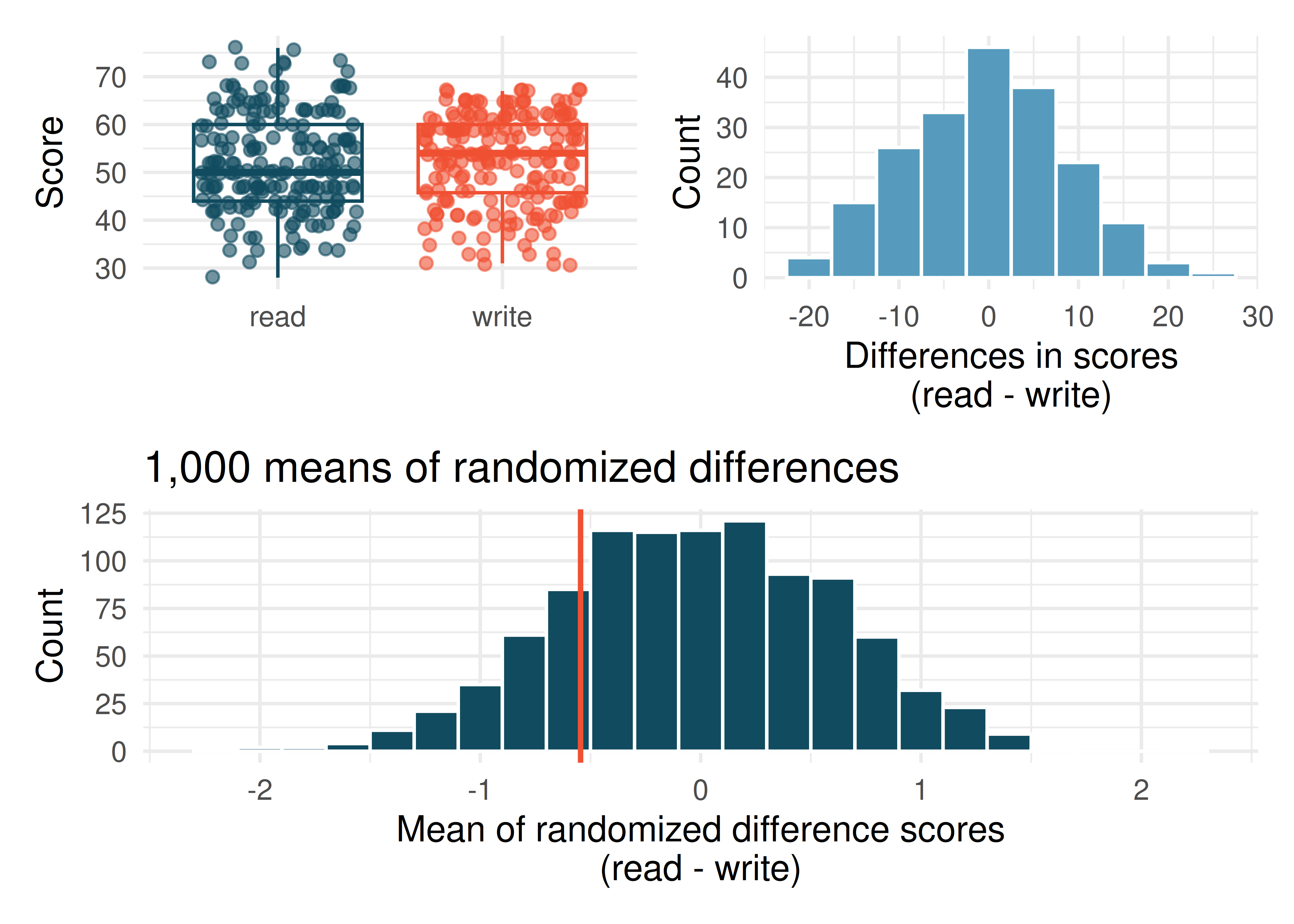
- High School and Beyond, randomization test. The National Center of Education Statistics conducted a survey of high school seniors, collecting test data on reading, writing, and several other subjects. Here we examine a simple random sample of 200 students from this survey.
Side-by-side box plots of reading and writing scores as well as a histogram of the differences in scores are shown below. Also provided below is a histogram of randomized averages of paired differences of scores (read - write), with the observed difference (\(\bar{x}_{read-write} = -0.545\)) marked with a red vertical line. The randomization distribution was produced by doing the following 1000 times: for each student, the two scores were randomly assigned to either read or write, and the average was taken across all students in the sample.
Is there a clear difference in the average reading and writing scores?
Are the reading and writing scores of each student independent of each other?
Create hypotheses appropriate for the following research question: is there an evident difference in the average scores of students in the reading and writing exam?
Is the average of the observed difference in scores \((\bar{x}_{read-write} = -0.545)\) consistent with the distribution of randomized average differences? Explain.
Do these data provide convincing evidence of a difference between the average scores on the two exams? Estimate the p-value from the randomization test, and conclude the hypothesis test using words like “score on reading test” and “score on writing test.”
- Global warming, randomization test. Let’s consider a limited set of climate data, examining temperature differences in 1950 vs 2022. We sampled 26 locations in the US from the National Oceanic and Atmospheric Administration’s (NOAA) historical data, where the data was available for both years of interest. (NOAA 2023) The data are not a random sample, but they are selected to be a representative sample across the land area of the lower 48 United States. Using the hottest day of the year as a measure can make the results susceptible to outliers. Instead, to get a sense for how hot a year was, we calculate the 90\(^{th}\) percentile; that is, we find the maximum temperature on the day that was hotter than 90% of the days that year. We want to know: is the 90\(^{th}\) percentile high temperature greater in 2022 or in 1950? The difference in 90\(^{th}\) percentile high temperature (high temperature for 2022 - high temperature for 1950) was calculated for each of the 26 locations. The average of the 26 differences was 2.52\(^\circ\)F with a standard deviation of 2.95\(^\circ\)F. We are interested in determining whether these data provide strong evidence that the 90\(^{th}\) percentile high temperature is higher in 2022 than in 1950.
Create hypotheses appropriate for the following research question: is there an evident difference in the 90\(^{th}\) percentile high temp across the two years (1950 and 2022)?
Is the average of the observed difference in scores \((\bar{x}_{2022-1950} = 2.53\)^\(F)\) consistent with the distribution of randomized average differences? Explain.
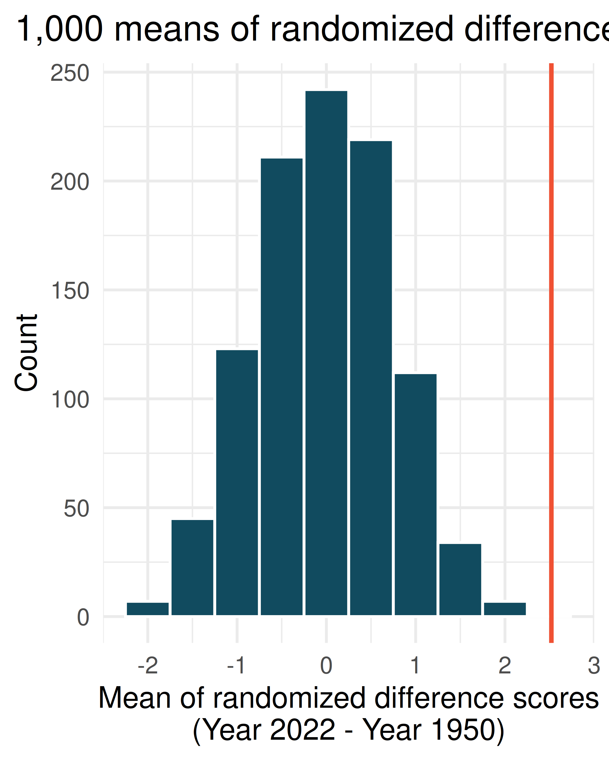
- Do these data provide convincing evidence of a difference between the 90\(^{th}\) percentile high temperature? Estimate the p-value from the randomization test, and conclude the hypothesis test using words like “90\(^{th}\) percentile high temperature in 1950” and “90\(^{th}\) percentile high temperature in 2022.”
- High School and Beyond, mathematical test. We considered the differences between the reading and writing scores of a random sample of 200 students who took the High School and Beyond Survey.
Create hypotheses appropriate for the following research question: is there an evident difference in the average scores of students in the reading and writing exam?
Check the conditions required to complete this test.
The average observed difference in scores is \(\bar{x}_{read-write} = -0.545\), and the standard deviation of the differences is \(s_{read-write} = 8.887\) points. Do these data provide convincing evidence of a difference between the average scores on the two exams?
What type of error might we have made? Explain what the error means in the context of the application.
Based on the results of this hypothesis test, would you expect a confidence interval for the average difference between the reading and writing scores to include 0? Explain your reasoning.
- Global warming, mathematical test. We considered the change in the 90\(^{th}\) percentile high temperature in 1950 versus 2022 at 26 sampled locations from the NOAA database. (NOAA 2023) The mean and standard deviation of the reported differences are 2.53\(^\circ\)F and 2.95\(^\circ\)F.
Is there a relationship between the observations collected in 1950 and 2022? Or are the observations in the two groups independent? Explain your reasoning.
Write hypotheses for this research in symbols and in words.
Check the conditions required to complete this test.
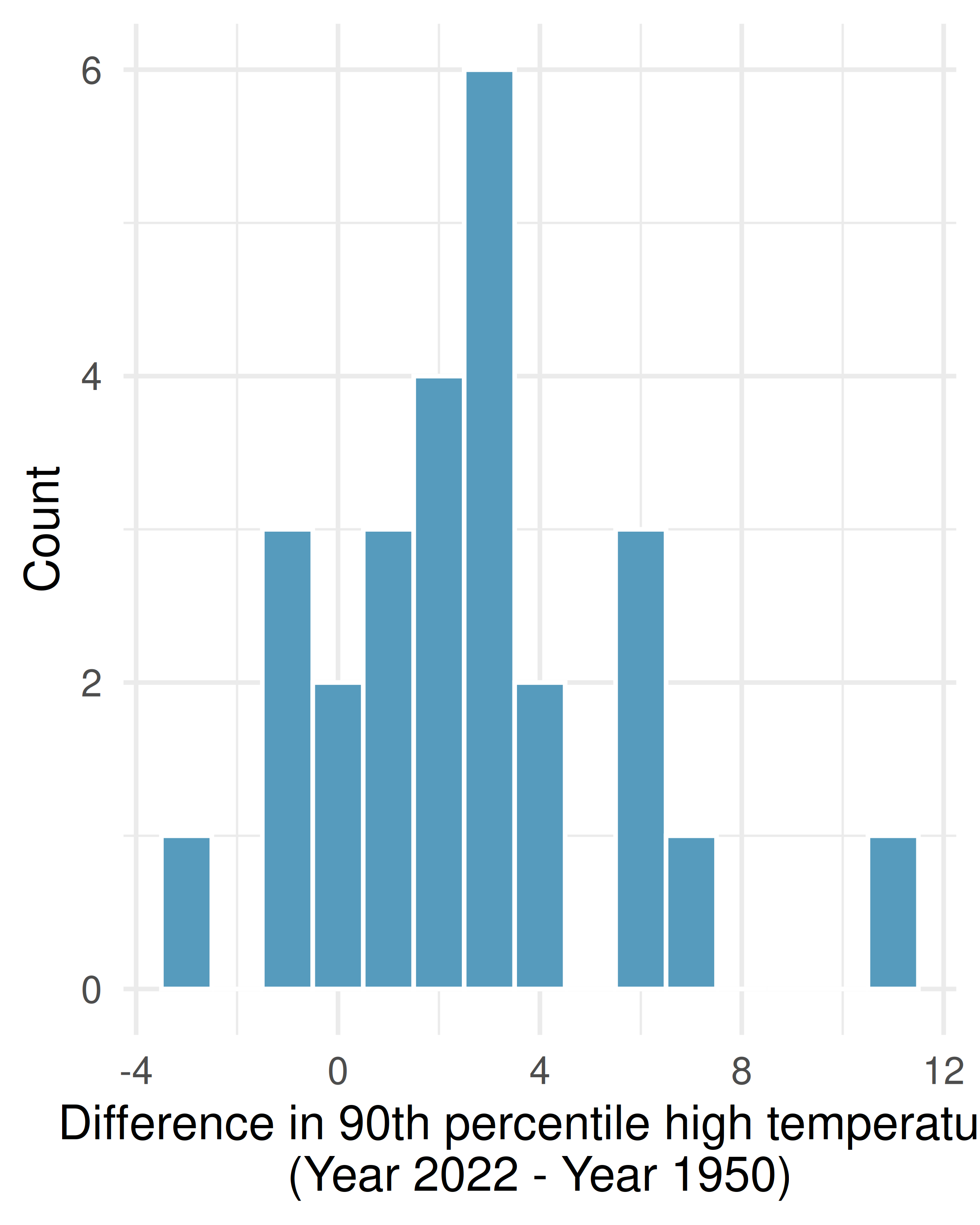
Calculate the test statistic and find the p-value.
Use \(\alpha = 0.05\) to evaluate the test, and interpret your conclusion in context.
What type of error might we have made? Explain in context what the error means.
Based on the results of this hypothesis test, would you expect a confidence interval for the average difference between the 90\(^{th}\) percentile high temperture from 1950 to 2022 to include 0? Explain your reasoning.
- Possible paired randomized differences. Two observations were collected on each of five people. Which of the following could be a possible randomization of the paired differences given in the table below? If the set of values could not be a randomized set of differences, indicate why not.
-2, 1, 1, 11, -2
-4, 11, -2, 0, 1
-2, 2, -11, 11, -2, 2, 0, 1, -1
0, -1, 2, -4, 11
4, -11, 2, 0, -1
| 1 | 2 | 3 | 4 | 5 | |
|---|---|---|---|---|---|
| Observation 1 | 3 | 14 | 4 | 5 | 10 |
| Observation 2 | 7 | 3 | 6 | 5 | 9 |
| Difference | -4 | 11 | -2 | 0 | 1 |
- Study environment. In order to test the effects of listening to music while studying versus studying in silence, students agree to be randomized to two treatments (i.e., study with music or study in silence). There are two exams during the semester, so the researchers can either randomize the students to have one exam with music and one with silence (randomly selecting which exam corresponds to which study environment) or the researchers can randomize the students to one study habit for both exams.
The researchers are interested in estimating the true population difference of exam score for those who listen to music while studying as compared to those who study in silence.
Describe the experiment which is consistent with a paired designed experiment. How is the treatment assigned, and how are the data collected such that the observations are paired?
Describe the experiment which is consistent with an indpenedent samples experiment. How is the treatment assigned, and how are the data collected such that the observations are independent?
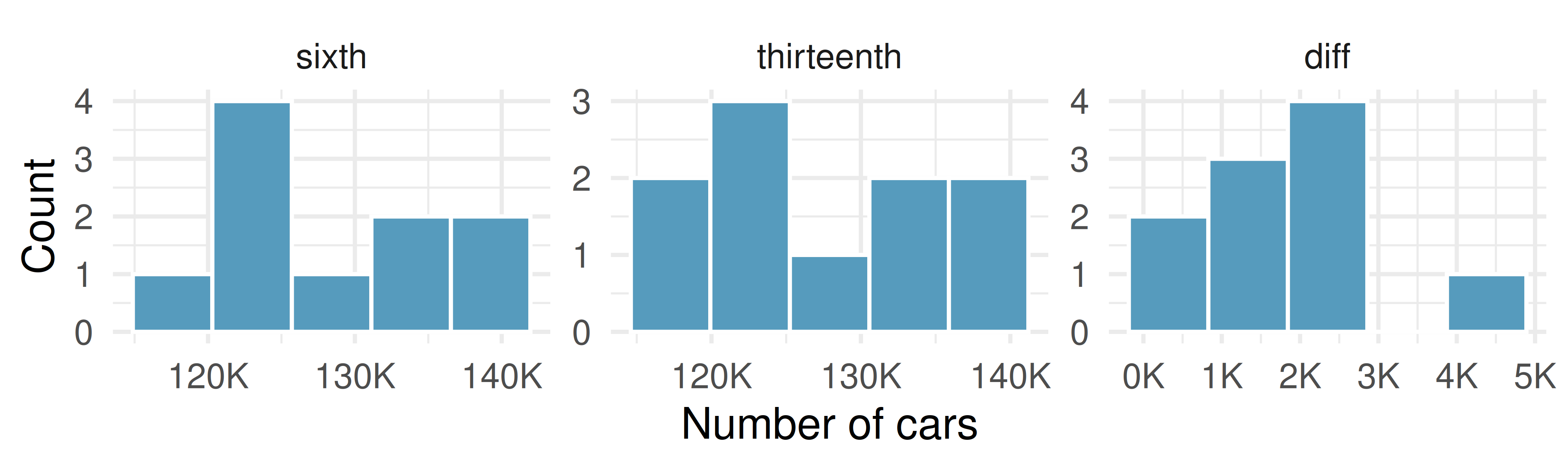
- Friday the 13th, traffic. In the early 1990’s, researchers in the UK collected data on traffic flow on Friday the 13th with the goal of addressing issues of how superstitions regarding Friday the 13th affect human behavior and and whether Friday the 13th is an unlucky day. The histograms below show the distributions of numbers of cars passing by a specific intersection on Friday the 6th and Friday the 13th for many such date pairs. Also provided are some sample statistics, where the difference is the number of cars on the 6th minus the number of cars on the 13th. (Scanlon et al. 1993)
| n | Mean | SD | |
|---|---|---|---|
| sixth | 10 | 128,385 | 7,259 |
| thirteenth | 10 | 126,550 | 7,664 |
| diff | 10 | 1,836 | 1,176 |
Are there any underlying structures in these data that should be considered in an analysis? Explain.
What are the hypotheses for evaluating whether the number of people out on Friday the 6\(^{\text{th}}\) is different than the number out on Friday the 13\(^{\text{th}}\)?
Check conditions to carry out the hypothesis test from part (b) using mathematical models.
Calculate the test statistic and the p-value.
What is the conclusion of the hypothesis test?
Interpret the p-value in this context.
What type of error might have been made in the conclusion of your test? Explain.
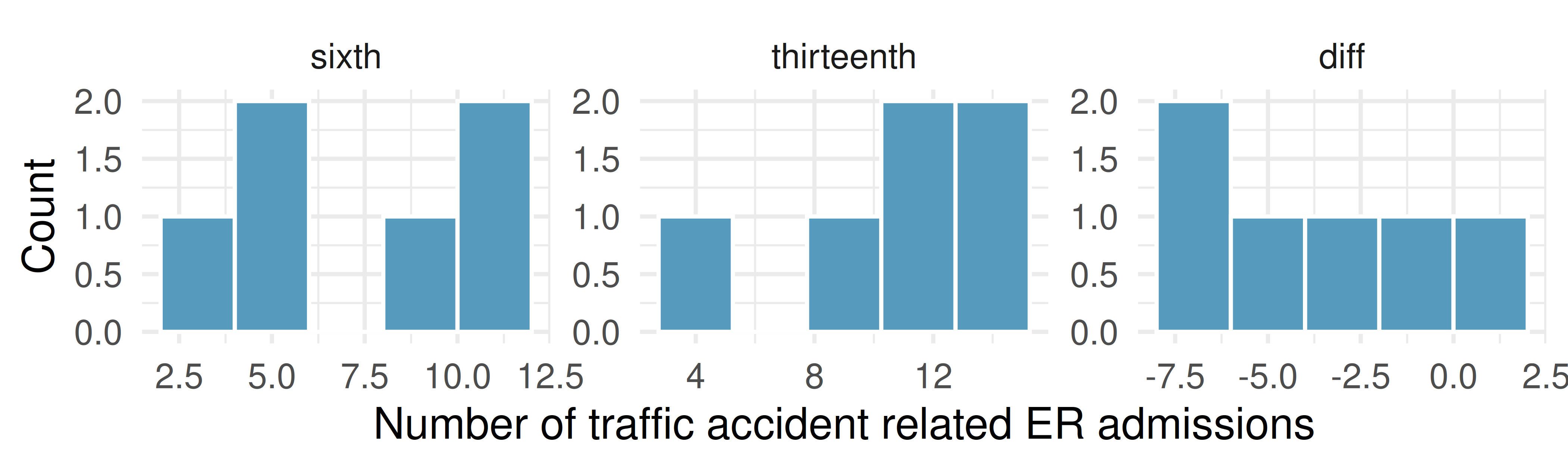
- Friday the 13th, accidents. In the early 1990’s, researchers in the UK collected data the number of traffic accident related emergency room (ER) admissions on Friday the 13th with the goal of addressing issues of how superstitions regarding Friday the 13th affect human behavior and and whether Friday the 13th is an unlucky day. The histograms below show the distributions of numbers of ER admissions at specific emergency rooms on Friday the 6th and Friday the 13th for many such date pairs. Also provided are some sample statistics, where the difference is the ER admissions on the 6th minus the ER admissions on the 13th.(Scanlon et al. 1993)
| n | Mean | SD | |
|---|---|---|---|
| sixth | 6 | 8 | 3 |
| thirteenth | 6 | 11 | 4 |
| diff | 6 | -3 | 3 |
Conduct a hypothesis test using mathematical models to evaluate if there is a difference between the average numbers of traffic accident related emergency room admissions between Friday the 6\(^{\text{th}}\) and Friday the 13\(^{\text{th}}\).
Calculate a 95% confidence interval using mathematical models for the difference between the average numbers of traffic accident related emergency room admissions between Friday the 6\(^{\text{th}}\) and Friday the 13\(^{\text{th}}\).
The conclusion of the original study states, “Friday 13th is unlucky for some. The risk of hospital admission as a result of a transport accident may be increased by as much as 52%. Staying at home is recommended.” Do you agree with this statement? Explain your reasoning.
Dataset sources
births14 (openintro) | diamonds (ggplot2) | lizard_run (openintro) | chickwts (datasets) | epa2021 (openintro) | hsb2 (openintro) | us_temperature (openintro) | friday (openintro)
StatLens Exercises
These exercises focus on the parts of inference a calculator can’t do for you: framing the question, choosing the right procedure, checking conditions, and interpreting what a tool reports. Where a link is given, let StatLens do the arithmetic and spend your effort on the reasoning.
Frame the question. A manufacturer advertises that its energy bars contain a mean of 220 calories. A consumer group buys a random sample of \(n = 36\) bars and measures the actual calorie content of each.
- Identify the parameter of interest in words and give its symbol.
- Write the null and alternative hypotheses for a test of whether the true mean differs from 220. Is your test one-sided or two-sided, and why?
- Suppose the consumer group instead suspected the manufacturer was under-filling the bars. Rewrite the alternative hypothesis. What is the practical danger of switching from a two-sided to a one-sided test after looking at the data?
Choose the procedure. For each scenario, name the procedure — one-sample \(t\), two-sample \(t\) (independent groups), paired \(t\), or a procedure beyond this chapter (more than two means, or a proportion).
- Each of 20 patients has their blood pressure measured before and after a meditation program; ask whether the program lowers blood pressure on average.
- An agronomist compares the mean yield (bushels/acre) of two corn varieties planted in 30 randomly chosen plots each.
- Is the proportion of voters who support a candidate more than 50%?
- Test whether the mean fuel economy of a single car model differs from the EPA-rated 32 mpg.
- Compare the mean weight gain of mice on three different diets.
Check conditions before you trust the test. Open the One-Sample \(t\) tool with any small numeric dataset (or paste in \(n = 15\) values of your own).
- What two conditions does the one-sample \(t\)-test require? State each in plain language.
- The tool displays a dotplot or histogram of the data alongside the \(t\)-statistic. With \(n = 15\), what would you look for in that picture to decide whether the test is trustworthy?
- Suppose the data show an extreme outlier — one observation more than three SDs from the rest. Should you still run the \(t\)-test? What two questions should you ask before deciding what to do with the outlier?
Run it and interpret it (two means). Open the Two-Sample \(t\) tool with any two-group numeric dataset (or use the bundled examples).
Identify the explanatory and response variables, and define \(\mu_1 - \mu_2\) in words.
Run the test. Report the test statistic, degrees of freedom, and p-value. State your decision at \(\alpha = 0.05\).
Write a one-sentence conclusion in context. Then write another sentence that translates the p-value into plain language — without using the words “probability that \(H_0\) is true.”
Which statement is the correct interpretation of the p-value?
- The probability that the null hypothesis is true given the data.
- The probability of observing a difference at least as extreme as the one we got, if \(H_0\) were true.
- The probability that \(\mu_1 = \mu_2\).
Simulation vs. analytic — when do they agree? A randomization test and a two-sample \(t\)-test are two routes to the same conclusion about whether two group means differ. Sometimes they land in nearly the same place; sometimes they don’t.
First a well-behaved case. Open any moderate-\(n\) two-group numeric dataset in the Two-Sample \(t\) tool and record the p-value, then open the same data in the Randomization Test for the Difference in Means and run 1000 shuffles.
- How close are the two p-values?
Now construct (or pick) a trouble case — a small dataset (\(n_1, n_2 \le 10\) each) where one group has a visible outlier or a strong skew. Run both procedures again.
- Are the p-values still close? Where do they diverge — is the \(t\)-test’s p-value smaller or larger than the randomization p-value? In which direction?
- Explain the pattern. Why do the two procedures agree on well-behaved data but diverge in the trouble case? Tie your explanation to (i) the role of normality in the \(t\) distribution and (ii) what the randomization test does assume (only exchangeability under \(H_0\)).
- A student says, “The randomization test gave a bigger p-value, so the \(t\)-test must be wrong.” Why is that the wrong framing? Which test should you trust more when they disagree, and why?
Adolph, S. C. 1987. “Physiological and Behavioral Ecology of the Lizards Sceloporus Occidentalis and Sceloporus Graciosus.” PhD thesis, University of Washington, Seattle, Washington.
McNeil, D. R. 1977. “Interactive Data Analysis: A Practical Primer.”
Mortada, WI, MA Sobh, MM El-Defrawy, and SE Farahat. 2000. “Study of Lead Exposure from Automobile Exhaust as a Risk for Nephrotoxicity Among Traffic Policemen.” American Journal of Nephrology 21 (4): 274–79. https://doi.org/10.1159/000046261.
NOAA. 2023. “Climate Data Online.” http://www.openintro.org/redirect.php?go=textbook-noaa_1948_2018.
Oldham-Cooper, R. E., C. A. Hardman, C. E. Nicoll, P. J. Rogers, and J. M. Brunstrom. 2011. “Playing a Computer Game During Lunch Affects Fullness, Memory for Lunch, and Later Snack Intake.” The American Journal of Clinical Nutrition 93 (2): 308. https://doi.org/10.3945/ajcn.110.004580.
Othman, S., N. Hassan, and A. Mohamed. 2023. “Effectiveness of Mindfulness-Based Interventions on Burnout and Self-Compassion Among Critical Care Nurses Caring for Patients with COVID-19: A Quasi-Experimental Study.” BMC Nursing 22: 35.
Scanlon, T. J., R. N. Luben, F. L. Scanlon, and N. Singleton. 1993. “Is Friday the 13th Bad for Your Health?” British Medical Journal 307: 1584–86. https://doi.org/10.1136/bmj.307.6919.1584.
US DOE EPA. 2021. “Fuel Economy, 2021 Data File.” https://www.openintro.org/go?id=textbook-fueleconomy-2021.
Wickham, H. 2016. ggplot2: Elegant Graphics for Data Analysis. Springer-Verlag New York. https://ggplot2.tidyverse.org.