10 Sampling Distributions via Simulation
In the randomization tests and bootstrap confidence intervals chapters, we used simulation to answer two fundamental questions of inference: Is there an effect? (randomization tests) and How big is the parameter? (bootstrap confidence intervals). Both methods relied on the computer to generate distributions — randomization distributions and bootstrap distributions — that helped us quantify uncertainty. In this chapter, we step back to see the bigger picture. We examine the shape, center, and spread of these simulated distributions and discover a remarkable pattern: under certain conditions, they all look approximately normal (bell-shaped). This observation, formalized as the Central Limit Theorem, is the bridge from the simulation-based methods of Unit 2 to the formula-based methods of Unit 3.
10.1 From simulation to theory
In the randomization tests and bootstrap confidence intervals chapters, we encountered several case studies:
- Sex discrimination (the randomization tests chapter): We shuffled promotion decisions and computed the difference in promotion rates 100 times.
- Opportunity cost (the randomization tests chapter): We shuffled buying decisions and computed the difference in proportions 1,000 times.
- Medical consultant (the bootstrap confidence intervals chapter): We bootstrapped the complication rate from 62 surgeries 10,000 times.
- Tappers and listeners (the bootstrap confidence intervals chapter): We bootstrapped the proportion of correct guesses from 120 listeners 10,000 times.
Each of these simulations produced a distribution of a sample statistic. While they differed in their settings, outcomes, and the simulation technique used, they all shared something in common: the general shape of the distribution.
Think back to the randomization and bootstrap distributions you have seen. What shape did most of them have? Were they skewed, uniform, or something else?
Show answer
In general, the distributions were approximately symmetric and bell-shaped. The two bootstrap distributions for small proportions — the medical consultant and the tappers and listeners — were the exceptions, with noticeable right skew, which makes sense because those proportions were very close to zero.This is no coincidence. The bell shape keeps appearing because of a deep mathematical result that underlies most of statistics. Whether we shuffle labels, resample with replacement, or imagine taking repeated samples from a population, the distribution of the resulting statistic tends to look the same — symmetric, unimodal, and bell-shaped.
In the simulation chapters, we let the computer show us this pattern directly. Now, we formalize it.
10.2 The Central Limit Theorem
The Central Limit Theorem (CLT) states that when we take sufficiently large random samples from a population, the sampling distribution of many common statistics (such as \(\hat{p}\) or \(\bar{x}\)) is approximately normal (bell-shaped), regardless of the shape of the underlying population distribution.
This is a stunning result. Even if the population distribution is skewed, bimodal, or has some other non-normal shape, the distribution of the sample statistic will be approximately normal — provided the sample is large enough.
Central Limit Theorem: the key ideas.
- The sampling distribution of a sample statistic is approximately normal when the sample size is large enough.
- The center of the sampling distribution is at the population parameter.
- The spread of the sampling distribution (the standard error) decreases as sample size increases.
These three facts together mean: with a large enough sample, the sample statistic will be close to the population parameter, and we can use the normal distribution to describe how close.
10.2.1 Conditions for the CLT
The normal approximation does not apply in all situations. Two conditions must hold:
Independent observations. The observations in the sample must be independent of each other. This is typically guaranteed by random sampling from a population, or by random assignment in an experiment.
Large enough sample. The sample size cannot be too small. What counts as “large enough” depends on the context:
- For proportions: we generally need at least 10 expected successes and 10 expected failures.
- For means: the rule of thumb depends on how skewed the population is. For roughly symmetric populations, \(n \geq 30\) is often sufficient. For highly skewed populations, larger samples may be needed.
When these conditions are not met, the normal approximation may be poor and simulation-based methods (randomization tests, bootstrap CIs) are the better choice. This is one of the great advantages of simulation: it works even when mathematical conditions are not satisfied.
10.2.2 Visualizing the CLT
Imagine a population that is distinctly non-normal — say, a right-skewed distribution like household income. If we take a single random sample of \(n = 5\) people and compute the mean income, that mean might be quite far from the population mean \(\mu\). But if we do this thousands of times (each time taking a new sample of 5 and computing the mean), the distribution of those thousands of sample means will already start to look somewhat bell-shaped, even though the underlying population is skewed.
Now increase the sample size to \(n = 30\). The distribution of sample means looks even more bell-shaped. At \(n = 100\), it is nearly indistinguishable from a perfect normal curve.
This progression — from skewed population, to somewhat normal at small \(n\), to very normal at larger \(n\) — is the Central Limit Theorem in action.
| Sample size | Shape of sampling distribution |
|---|---|
| \(n = 5\) | Retains some skew from the population |
| \(n = 30\) | Approximately normal for most populations |
| \(n = 100\) | Very close to normal for virtually all populations |
The speed at which the sampling distribution approaches normality depends on how non-normal the population is. Symmetric populations converge quickly; highly skewed populations take longer.
Predict → Do → Explain. Open the Sampling Distribution Lab to watch the CLT emerge from a strongly right-skewed population. The gated activity opens with a Predict step (commit to where the sample means will pile up when the population is skewed), walks you through drawing samples of \(n = 10\) and then freezing that picture to compare it with \(n = 100\) on a shared axis, and closes with an Explain step where you put the Central Limit Theorem in your own words — why the sampling distribution centers at \(\mu\) and turns bell-shaped, and why a larger \(n\) shrinks the spread but does not move the center. Your predictions and explanation save locally in the tool, so you can return to your work on the same device.
10.3 Comparing randomization, bootstrap, and mathematical approaches
We now have three tools for statistical inference, each grounded in the same core ideas but using different mechanisms:
| Randomization | Bootstrap | Mathematical model | |
|---|---|---|---|
| Question answered | Is there an effect? (hypothesis test) | How big is the parameter? (confidence interval) | Both |
| How variability is generated | Shuffle labels to simulate \(H_0\) | Resample with replacement from sample | Use formulas based on the normal distribution |
| What it models | Variability due to random assignment | Variability due to random sampling | Variability predicted by mathematical theory |
| Center of distribution | Null hypothesis value | Sample statistic | Depends on context (\(H_0\) for tests, \(\hat{p}\) for CIs) |
| Conditions required | Minimal | Minimal | Independence + large sample |
| Computational cost | Moderate (need many simulations) | Moderate (need many resamples) | Low (just plug into formula) |
Key insight. All three methods answer the same fundamental question: How much does the statistic vary? They just measure that variability in different ways.
- Randomization asks: “How much would the statistic vary if the null hypothesis were true?”
- Bootstrap asks: “How much would the statistic vary across different samples from this population?”
- Mathematical models ask: “How much does theory predict the statistic would vary?”
When conditions are met, all three give similar answers. The mathematical approach is faster and requires no simulation, which is why it is widely used. But the simulation approaches are more flexible and work even when conditions for the mathematical model are not met.
10.3.1 Which method should I use?
Here is a practical guide:
When conditions for the mathematical model are clearly met (independent observations, large sample, not too skewed), the formula-based approach is convenient and widely accepted. This will be our primary tool in Unit 3.
When conditions are questionable (small sample, very skewed data, unusual statistic), simulation-based methods are safer. The bootstrap and randomization test make fewer assumptions.
When you want to build intuition, simulation is invaluable. Seeing 10,000 shuffles or resamples gives you a concrete feel for what “random variability” looks like — something a formula alone cannot provide.
In practice, many statisticians use simulation to check their formula-based results. If the two approaches agree, confidence in the conclusion is strengthened.
10.4 When is the normal approximation good enough?
The mathematical approach to inference (which we will develop in Unit 3) replaces simulation with the normal distribution. Instead of generating thousands of shuffles or resamples, we use a formula to compute the standard error and then rely on the bell curve to find \(p\)-values or construct confidence intervals.
But when can we trust this shortcut?
10.4.1 The success-failure condition for proportions
For a sample proportion \(\hat{p}\), the sampling distribution is approximately normal when:
\[np \geq 10 \quad \text{and} \quad n(1 - p) \geq 10\]
where \(n\) is the sample size and \(p\) is the proportion of interest. In practice, since \(p\) is unknown, we use \(\hat{p}\) as a stand-in:
\[n\hat{p} \geq 10 \quad \text{and} \quad n(1 - \hat{p}) \geq 10\]
This is called the success-failure condition.
In the medical consultant example, \(n = 62\) and \(\hat{p} = 3/62 = 0.048\). Check the success-failure condition.
- Expected successes: \(n\hat{p} = 62 \times 0.048 = 3\) (less than 10)
- Expected failures: \(n(1 - \hat{p}) = 62 \times 0.952 = 59\) (at least 10)
The success-failure condition is not met because there are fewer than 10 expected successes. The normal approximation would be unreliable here. This is exactly the kind of situation where the bootstrap (as used in the bootstrap confidence intervals chapter) is the better approach.
In the tappers and listeners study, \(n = 120\) and \(\hat{p} = 3/120 = 0.025\). Check the success-failure condition. Should we use the normal approximation?
Show answer
Expected successes: \(120 \times 0.025 = 3\) (less than 10). Expected failures: \(120 \times 0.975 = 117\) (at least 10). The condition is not met because there are too few successes. The normal approximation would not be appropriate. Bootstrap methods are preferred.A poll of \(n = 1{,}000\) voters finds that \(\hat{p} = 0.52\) support a policy. Check the success-failure condition.
- Expected successes: \(n\hat{p} = 1{,}000 \times 0.52 = 520\) (well above 10)
- Expected failures: \(n(1 - \hat{p}) = 1{,}000 \times 0.48 = 480\) (well above 10)
The success-failure condition is comfortably met. The normal approximation is reliable here.
10.4.2 The sample size condition for means
For a sample mean \(\bar{x}\), the CLT tells us the sampling distribution is approximately normal when:
- The sample size is “large enough,” and
- The observations are independent.
A common guideline is \(n \geq 30\), but this is only a rough rule of thumb. If the population distribution is nearly symmetric, the normal approximation can work well even for smaller samples. If the population is highly skewed or has extreme outliers, a larger sample may be needed.
| Population shape | Minimum \(n\) for normal approximation |
|---|---|
| Symmetric, no outliers | \(n \geq 15\) or even smaller |
| Slightly skewed | \(n \geq 30\) |
| Highly skewed or heavy-tailed | \(n \geq 60\) or more |
When in doubt, use simulation (bootstrap) to check whether the normal approximation is reasonable.
10.4.3 Simulation as a check on theory
One of the most powerful uses of simulation is as a reality check on mathematical results. Here is the workflow:
- Compute a confidence interval or \(p\)-value using the formula-based (normal) approach.
- Compute the same quantity using simulation (bootstrap CI or randomization test).
- Compare. If the two results are similar, you can be confident in the mathematical approach. If they differ substantially, the conditions for the normal approximation may not be met, and you should rely on the simulation result.
This “trust but verify” approach is standard practice among professional statisticians and data scientists.
10.5 The normal distribution: a preview
Since the normal distribution will be our primary tool in Unit 3, let us briefly introduce its key features here.
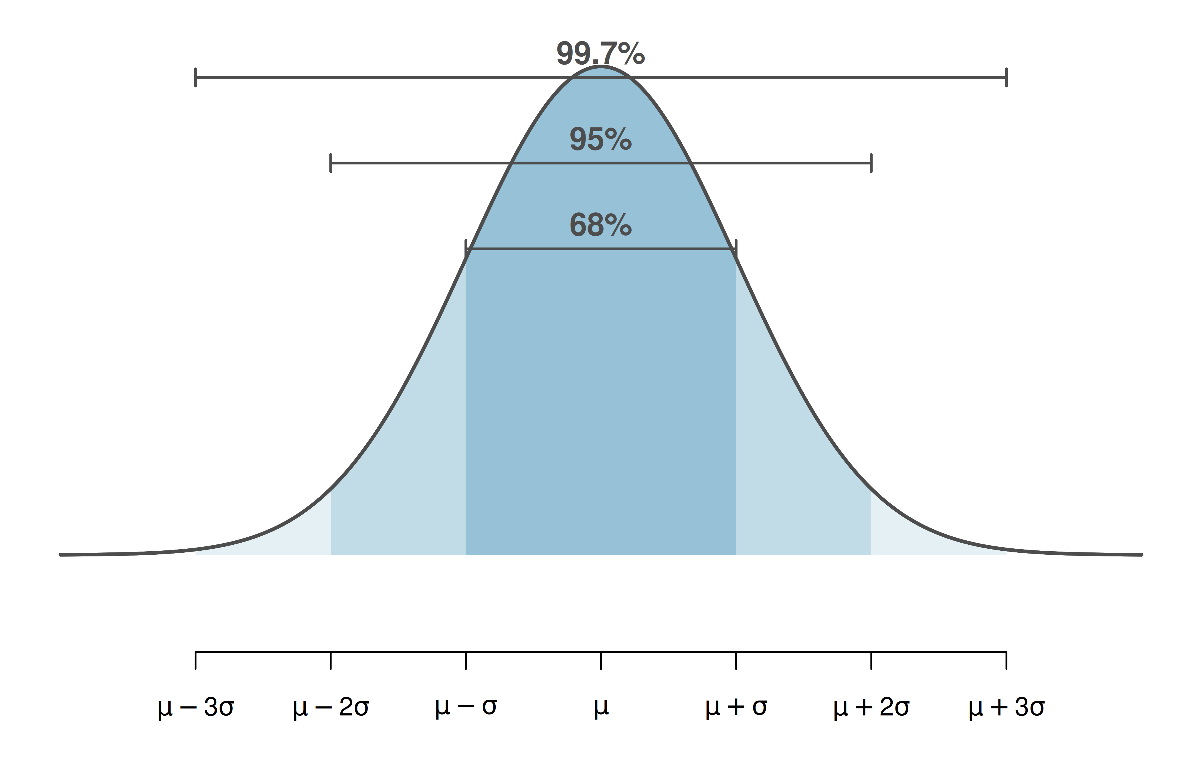
10.5.1 The 68-95-99.7 rule
The normal distribution has a very useful property: the percentage of observations falling within 1, 2, and 3 standard deviations of the mean is always approximately the same.
The 68-95-99.7 rule.
For any normal distribution:
- About 68% of values fall within 1 standard deviation of the mean: \(\mu \pm \sigma\)
- About 95% of values fall within 2 standard deviations of the mean: \(\mu \pm 2\sigma\)
- About 99.7% of values fall within 3 standard deviations of the mean: \(\mu \pm 3\sigma\)
This rule is the reason behind the quick approximation we already met in the bootstrap confidence intervals chapter: a 95% confidence interval \(\approx\) statistic \(\pm\, 2 \times SE\). We used it there; now we can see why it works — when the bootstrap (or sampling) distribution is roughly normal, its middle 95% lies within about 2 standard deviations, which for a statistic means about 2 standard errors:
\[\text{95\% CI} \approx \text{statistic} \pm 2 \times SE\]
A poll of \(n = 1{,}000\) voters finds \(\hat{p} = 0.52\) with a standard error of \(SE = 0.016\). Use the quick approximation to construct a 95% confidence interval.
\[\hat{p} \pm 2 \times SE = 0.52 \pm 2(0.016) = 0.52 \pm 0.032 = (0.488, 0.552)\]
We are 95% confident that the true proportion of voters who support the policy is between 48.8% and 55.2%.
Why is it “approximately 2” standard errors rather than exactly 2? What is the more precise multiplier for a 95% confidence interval based on the normal distribution?
Show answer
The more precise multiplier is 1.96, not 2. The value 1.96 is the Z-score that puts exactly 2.5% in each tail of the standard normal distribution, leaving 95% in the middle. The approximation of 2 is close enough for quick mental calculations.10.5.2 Z scores
A Z score measures how many standard deviations an observation is above or below the mean:
\[Z = \frac{x - \mu}{\sigma}\]
In the context of sampling distributions, we can compute a Z score for an observed statistic:
\[Z = \frac{\text{statistic} - \text{parameter}}{SE}\]
This Z score tells us how unusual the observed statistic is, measured in standard-error units. In Unit 3, we will use Z scores (and their cousins, t-scores) extensively to compute \(p\)-values and confidence intervals without simulation.
In the sex discrimination study, the observed difference in promotion rates was 0.292. Suppose the standard error of the difference (computed under the null hypothesis) is 0.12. Compute the Z score.
Under \(H_0\), the parameter (the true difference) is 0. So:
\[Z = \frac{0.292 - 0}{0.12} = 2.43\]
The observed difference is 2.43 standard errors above the null value of 0. Since values beyond 2 standard deviations are unusual for a normal distribution (the 95% rule), this is strong evidence against the null hypothesis — consistent with our earlier simulation result.
10.6 Recap: connecting the three approaches
Types of distributions (a reference guide).
You have now encountered several types of distributions in this course. Understanding the differences among them is essential:
- A data distribution (or sample distribution) describes the shape, center, and variability of the observed data.
- A population distribution describes the entire population — almost always unknown.
- A sampling distribution describes how a sample statistic varies from sample to sample. The CLT tells us this is approximately normal under certain conditions.
- A randomization distribution describes how a sample statistic varies under random shuffling of the treatment variable. It is centered at the null hypothesis value.
- A bootstrap distribution describes how a statistic varies under resampling from the observed data. It is centered at the observed statistic.
10.6.1 The big picture of Unit 2
Unit 2 has built your intuition for statistical inference using simulation:
| Chapter | Method | Question | How variability is generated |
|---|---|---|---|
| 6 | Sampling variability | How much do statistics vary? | Conceptual + simulation |
| 7 | Randomization test | Is there an effect? | Shuffle labels |
| 8 | Decision errors | How can a test go wrong? | Simulated Type I / Type II rates |
| 9 | Bootstrap CI | How big is the parameter? | Resample with replacement |
| 10 | CLT and normal model | Can we skip the simulation? | Mathematical formula |
The key takeaway: the simulation methods and the mathematical methods are answering the same questions. The CLT tells us when the mathematical shortcuts are valid. When they are, we can replace thousands of computer simulations with a single formula.
In Unit 3, we will develop these formula-based methods for specific settings: one proportion, one mean, two proportions, two means, and more. But you now have the conceptual foundation to understand why those formulas work: they are mathematical descriptions of the same sampling variability that you observed through simulation.
10.7 Chapter review
10.7.1 Summary
- Randomization distributions, bootstrap distributions, and theoretical sampling distributions all tend to be approximately bell-shaped (normal) under common conditions. This is the Central Limit Theorem (CLT).
- The CLT states that for sufficiently large samples with independent observations, the sampling distribution of many common statistics is approximately normal, regardless of the shape of the population.
- The success-failure condition (\(n\hat{p} \geq 10\) and \(n(1-\hat{p}) \geq 10\)) is the practical check for whether the normal approximation is appropriate for proportions.
- The 68-95-99.7 rule describes the area under a normal curve within 1, 2, and 3 standard deviations of the mean.
- A Z score measures how many standard deviations (or standard errors) an observation or statistic falls from the mean: \(Z = (x - \mu)/\sigma\).
- The three inference approaches — randomization, bootstrap, and mathematical models — answer the same fundamental questions. When conditions are met, they produce similar results. Mathematical models are faster; simulation methods are more flexible.
- This chapter bridges Unit 2 (simulation-based inference) and Unit 3 (formula-based inference). The CLT is the theoretical justification for the formulas we will use in Unit 3.
10.7.2 Key terms
| Term | Definition |
|---|---|
| Central Limit Theorem (CLT) | The sampling distribution of a statistic is approximately normal for large samples |
| Normal distribution | A symmetric, bell-shaped distribution described by its mean and standard deviation |
| Success-failure condition | For proportions: need \(n\hat{p} \geq 10\) and \(n(1-\hat{p}) \geq 10\) |
| 68-95-99.7 rule | About 68%, 95%, 99.7% of normal values fall within 1, 2, 3 SDs of the mean |
| Z score | Number of standard deviations an observation falls from the mean: \(Z = (x-\mu)/\sigma\) |
| Null distribution | The sampling distribution of the sample statistic under \(H_0\) |
| Sampling distribution | Distribution of a statistic over all possible samples of a given size |
10.8 Exercises
Answers to odd-numbered exercises are provided in the Exercise Solutions appendix at the back of the book.
- Repeated water samples. A nonprofit wants to understand the fraction of households that have elevated levels of lead in their drinking water. They expect at least 5% of homes will have elevated levels of lead, but not more than about 30%. They randomly sample 800 homes and work with the owners to retrieve water samples, and they compute the fraction of these homes with elevated lead levels. They repeat this 1,000 times and build a distribution of sample proportions.
What is this distribution called?
Would you expect the shape of this distribution to be symmetric, right skewed, or left skewed? Explain your reasoning.
What is the name of the variability of this distribution.
Suppose the researchers’ budget is reduced, and they are only able to collect 250 observations per sample, but they can still collect 1,000 samples. They build a new distribution of sample proportions. How will the variability of this new distribution compare to the variability of the distribution when each sample contained 800 observations?
- Repeated student samples. Of all freshman at a large college, 16% made the dean’s list in the current year. As part of a class project, students randomly sample 40 students and check if those students made the list. They repeat this 1,000 times and build a distribution of sample proportions.
What is this distribution called?
Would you expect the shape of this distribution to be symmetric, right skewed, or left skewed? Explain your reasoning.
What is the name of the variability of this distribution?
Suppose the students decide to sample again, this time collecting 90 students per sample, and they again collect 1,000 samples. They build a new distribution of sample proportions. How will the variability of this new distribution compare to the variability of the distribution when each sample contained 40 observations?
- Stating the Central Limit Theorem. The Central Limit Theorem (CLT) is one of the most important results in statistics. It says that for a random sample of independent observations \(X_1, X_2, \ldots, X_n\) drawn from a population with mean \(\mu\) and finite standard deviation \(\sigma\):
- The sampling distribution of the sample mean \(\bar{X}\) has mean \(\mu\),
- The sampling distribution of \(\bar{X}\) has standard deviation \(\sigma / \sqrt{n}\),
- As \(n\) grows, the shape of the sampling distribution of \(\bar{X}\) becomes approximately normal, regardless of the shape of the population.
A population of household incomes is strongly right-skewed. Which of the following are true according to the CLT? (Select all that apply — no justification needed.)
- As \(n\) grows, the sampling distribution of \(\bar{X}\) becomes approximately normal.
- As \(n\) grows, the population distribution becomes approximately normal.
- As \(n\) grows, the standard error \(\sigma/\sqrt{n}\) shrinks.
- As \(n\) grows, the population mean \(\mu\) changes.
A survey draws a random sample of \(n = 400\) students; call the sample mean GPA \(\bar{X}\). The population of student GPAs has mean \(\mu = 3.15\) and standard deviation \(\sigma = 0.60\). What are the approximate mean and standard error of the sampling distribution of \(\bar{X}\)?
A common misstatement of the CLT is: “When \(n\) is large, the sample data will be approximately normal.” Explain in one sentence why this is wrong.
Roughly how large does \(n\) need to be for the CLT to give a good approximation? Discuss briefly.
StatLens Exercises
Let StatLens do the arithmetic; spend your effort on the reasoning a calculator can’t do.
Predict, then check the CLT. Open the Sampling Distribution Lab and pick a right-skewed population.
- Before drawing anything: at \(n = 5\), do you expect the sampling distribution of \(\bar{x}\) to (i) match the shape of the population, (ii) look symmetric and bell-shaped, or (iii) look somewhere in between?
- Draw 5000 sample means at \(n = 5\). What shape do you actually see?
- Repeat at \(n = 30\) and \(n = 100\). At what point does the sampling distribution look “approximately normal” to your eye?
- Now switch the population to bimodal. At what \(n\) does the sampling distribution of \(\bar{x}\) start to look normal, compared to the right-skewed case?
More samples vs. larger \(n\) — which knob does what? Stay in the Sampling Distribution Lab with a right-skewed population at \(n = 10\).
- Draw 100 samples and note the spread (the displayed SD of the sample means). Then draw 5000 more (without changing \(n\)). Did the spread shrink?
- Now reset and start over at \(n = 40\). Draw 5000 samples. How does the spread compare to your \(n = 10\) run?
- Predict, without computing: if you go from \(n = 10\) to \(n = 40\), by what factor should the standard error of \(\bar{x}\) shrink? Check against what the lab reports for \(\sigma/\sqrt{n}\).
- A student says: “If I just draw enough samples, the standard error will eventually drop to zero.” Why is this wrong? What does drop to (essentially) zero with more samples?
Sampling distribution of \(\hat{p}\). Switch the Sampling Distribution Lab to proportion mode. Set the true population proportion to \(p = 0.20\) and the sample size to \(n = 20\).
- Predict the center and spread of the sampling distribution of \(\hat{p}\) (use \(\sqrt{p(1-p)/n}\) for the spread).
- Draw 5000 samples. Compare your predicted center and spread to the observed values. How close are they?
- Look at the shape of the sampling distribution. Is it symmetric or skewed? Why?
- Increase \(n\) to 200 (keep \(p = 0.20\)). Does the shape change? Use the success–failure rule (\(np \ge 10\), \(n(1-p) \ge 10\)) to predict what should happen at \(n = 200\) vs. \(n = 20\).
Reading sampling distributions in context. A factory produces light bulbs with mean lifetime \(\mu = 1000\) hours and standard deviation \(\sigma = 200\) hours. A quality engineer plans to take a random sample of \(n = 50\) bulbs and compute the sample mean lifetime \(\bar{x}\).
- What is the sampling distribution of \(\bar{x}\)? Give its mean, standard error, and shape (and justify the shape).
- What is the probability the sample mean is less than 950 hours? Use a normal distribution tool (pre-loaded with \(\mu = 1000\) and \(\sigma = 200/\sqrt{50} \approx 28.28\)).
- Suppose the engineer instead samples \(n = 200\) bulbs. Without re-running the tool, will the probability in (b) be smaller or larger? Why?
- An executive says: “The sample mean has the same distribution as a single bulb’s lifetime.” Why is this wrong, and what’s the impact on planning?
The CLT’s escape clauses — when do you not get normality? The CLT requires (i) an i.i.d. sample and (ii) a finite variance.
- Suppose 50 students at one cafeteria table sample sizes their lunches. Why is this not an i.i.d. sample for the population of students? What might go wrong if you computed a CLT-based interval for the mean lunch size?
- The Cauchy distribution has no defined mean or variance — it’s a heavy-tailed distribution. What would you expect to see if you drew sample means from a Cauchy population at \(n = 30\), \(n = 100\), \(n = 1000\)? (You can’t simulate this in the lab, but reason about it.)
- In practice, why is the violation in (a) (clustering / non-independence) much more common in real data than the violation in (b) (no finite variance)?
- Suppose you have \(n = 5000\) but the data come from social-media engagement (one big viral post can outweigh 4999 normal ones). Is the CLT comforting here? Why or why not?