24  Probability Rules

Probability forms the foundation of statistics, and you are probably already aware of many of the ideas we will discuss in this chapter. However, formalizing these concepts is likely new. While this chapter provides the theoretical foundation for the inference methods you have already been using, it also offers practical tools for reasoning about uncertainty. We will define probability, develop rules for combining probabilities, and explore conditional probability and independence — all concepts that underpin the inference methods from Parts II and III.

24.1 Defining probability

Statistics is built on probability, and probability gives us the language to describe uncertainty. We begin with a few simple examples that may feel familiar.

A “die,” the singular of “dice,” is a cube with six faces numbered 1, 2, 3, 4, 5, and 6. What is the chance of getting a 1 when rolling a fair die?

If the die is fair, then the chance of a 1 is as good as the chance of any other number. Since there are six equally likely outcomes, the chance must be 1-in-6 or, equivalently, \(1/6\).

What is the chance of getting a 1 or 2 on the next roll?

The outcomes 1 and 2 constitute two of the six equally likely outcomes, so the chance of getting one of these two is \(2/6 = 1/3\).

What is the chance of not rolling a 2?

Since the chance of rolling a 2 is \(1/6\), the chance of not rolling a 2 must be \(1 - 1/6 = 5/6\). Alternatively, not rolling a 2 means getting a 1, 3, 4, 5, or 6, which makes up five of the six equally likely outcomes.

We use probability to describe and understand apparent randomness. We frame probability in terms of a random process giving rise to an outcome.

Random process	Possible outcomes
Roll a die	1, 2, 3, 4, 5, or 6
Flip a coin	H or T

The probability of an outcome is the proportion of times the outcome would occur if we observed the random process an infinite number of times. Probability always takes values between 0 and 1 (inclusive) and may also be expressed as a percentage between 0% and 100%.

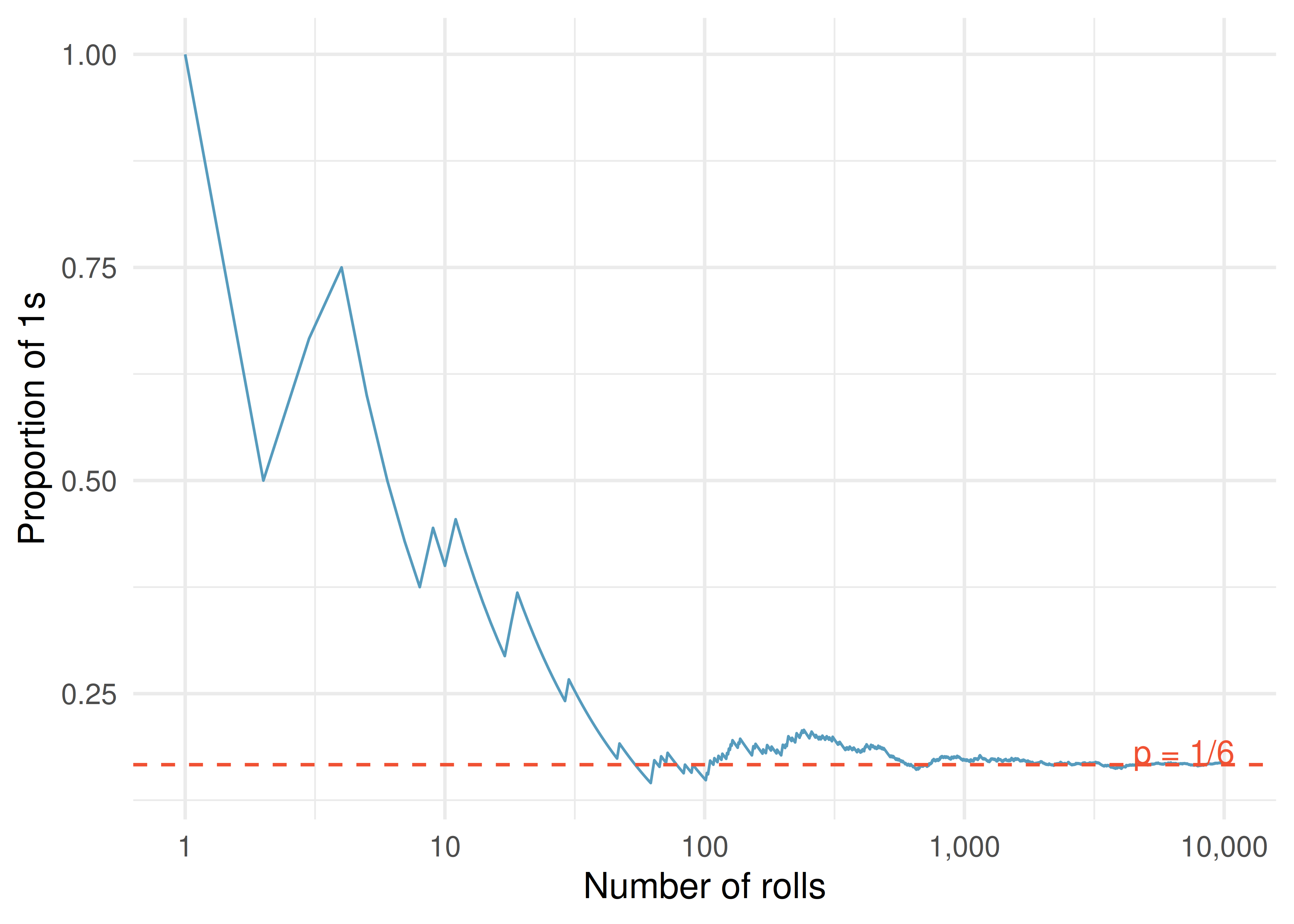
Probability can be illustrated by rolling a die many times. Let \(\hat{p}_n\) be the proportion of outcomes that are 1 after the first \(n\) rolls. As the number of rolls increases, \(\hat{p}_n\) converges to the probability \(p = 1/6\).

Figure 24.1: The fraction of die rolls that are 1 at each stage in a simulation. The proportion tends to get closer to 1/6 as the number of rolls increases.

Law of Large Numbers. As more observations are collected, the proportion \(\hat{p}_n\) of occurrences with a particular outcome converges to the probability \(p\) of that outcome.

Occasionally the proportion will veer away from the true probability, but these deviations become smaller as the number of trials increases.

We write the probability of rolling a 1 as \(P(\text{rolling a 1})\). When the context is clear, we abbreviate this as \(P(1)\).

Random processes include rolling a die and flipping a coin. (a) Think of another random process. (b) Describe all the possible outcomes of that process.

Show answer

1. and (b) Here are several examples. (i) Whether someone gets sick next month: outcomes are sick and not sick. (ii) Randomly selecting a person and measuring their height: the outcome is a positive number. (iii) Whether the stock market goes up or down next week: outcomes are up, down, and no change. (iv) The number of emails you receive tomorrow: the outcome is a non-negative integer.

24.1.1 Simulation: The law of large numbers in action

One of the most powerful ways to build intuition about probability is through simulation. Imagine writing a computer program that simulates flipping a fair coin 10,000 times and tracking the running proportion of heads after each flip.

• After 10 flips, the proportion of heads might be 0.30 or 0.70 — quite far from 0.50.
• After 100 flips, the proportion is likely between 0.40 and 0.60.
• After 1,000 flips, the proportion is usually between 0.47 and 0.53.
• After 10,000 flips, it is almost certainly within 0.01 of 0.50.

This is the Law of Large Numbers at work. The key insight is that probability is a long-run concept. In the short run, anything can happen. In the long run, patterns emerge with remarkable stability.

This simulation perspective will recur throughout our course. In Parts II and III, we used simulation to build sampling distributions and test hypotheses. Here in Unit 4, we develop the mathematical rules that explain why those simulations work.

24.2 Sample spaces and events

The sample space \(S\) of a random process is the set of all possible outcomes. An event is a subset of the sample space — that is, a collection of one or more outcomes.

For rolling a single die, the sample space is \(S = \{1, 2, 3, 4, 5, 6\}\).

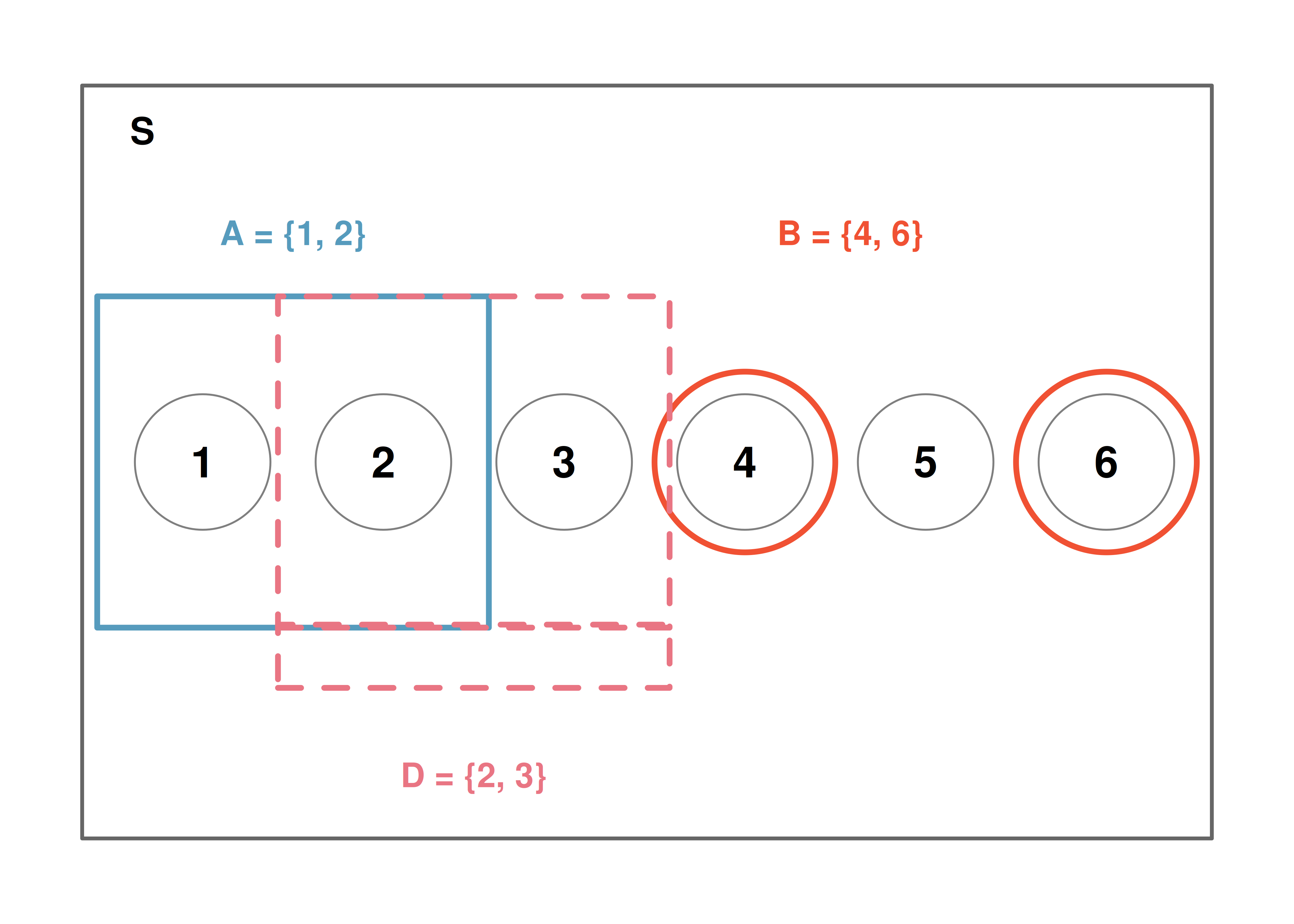
Let \(A\) represent the event that the die roll results in 1 or 2, so \(A = \{1, 2\}\). Let \(B\) represent the event that the die roll is 4 or 6, so \(B = \{4, 6\}\). These events are shown visually in the diagram below.

Figure 24.2: Three events for die outcomes. A and B are disjoint since they share no outcomes.

24.3 The complement rule

Let \(D = \{2, 3\}\) represent the event that the outcome of a die roll is 2 or 3. Then the complement of \(D\), denoted \(D^c\), represents all outcomes in the sample space that are not in \(D\):

\[D^c = \{1, 4, 5, 6\}\]

1. Compute \(P(D^c) = P(\text{rolling a 1, 4, 5, or 6})\). (b) What is \(P(D) + P(D^c)\)?

Show answer

1. The outcomes are disjoint and each has probability \(1/6\), so \(P(D^c) = 4/6 = 2/3\). (b) \(P(D) = 1/6 + 1/6 = 1/3\). Since \(D\) and \(D^c\) are disjoint, \(P(D) + P(D^c) = 1/3 + 2/3 = 1\).

A complement \(A^c\) is constructed so that (i) every possible outcome not in \(A\) is in \(A^c\), and (ii) \(A\) and \(A^c\) are disjoint. This gives us:

Complement rule. The complement of event \(A\) is denoted \(A^c\) and represents all outcomes not in \(A\). The probabilities of \(A\) and \(A^c\) are related by:

\[P(A) + P(A^c) = 1 \qquad \text{equivalently,} \qquad P(A) = 1 - P(A^c)\]

The complement rule is especially useful when computing a probability directly would be tedious but the complement is simple.

Let \(A\) represent the event where the sum of two dice is less than 12. What is \(P(A)\)?

The complement \(A^c\) is the event that the sum equals 12. The only way to roll a sum of 12 is to get two 6s, so \(P(A^c) = 1/36\). Using the complement rule:

\[P(A) = 1 - P(A^c) = 1 - \frac{1}{36} = \frac{35}{36}\]

Find the following probabilities for rolling two dice: (a) The sum is not 6. (b) The sum is at least 4. (c) The sum is no more than 10.

Show answer

1. \(P(\text{sum} = 6) = 5/36\), so \(P(\text{not 6}) = 1 - 5/36 = 31/36\). (b) \(P(\text{sum} = 2 \text{ or } 3) = 1/36 + 2/36 = 1/12\), so \(P(\text{at least 4}) = 1 - 1/12 = 11/12\). (c) \(P(\text{sum} = 11 \text{ or } 12) = 2/36 + 1/36 = 1/12\), so \(P(\text{no more than 10}) = 1 - 1/12 = 11/12\).

24.4 The addition rule

24.4.1 Disjoint (mutually exclusive) events

Two outcomes or events are called disjoint (or mutually exclusive) if they cannot both happen at the same time. For instance, when rolling a die, the outcomes 1 and 2 are disjoint since they cannot both occur on a single roll.

Addition rule for disjoint events. If \(A_1\) and \(A_2\) are disjoint events, then:

\[P(A_1 \text{ or } A_2) = P(A_1) + P(A_2)\]

More generally, if \(A_1, A_2, \ldots, A_k\) are all mutually disjoint, then:

\[P(A_1 \text{ or } A_2 \text{ or } \cdots \text{ or } A_k) = P(A_1) + P(A_2) + \cdots + P(A_k)\]

We are interested in the probability of rolling a 1, 4, or 5. (a) Explain why the outcomes 1, 4, and 5 are disjoint. (b) Apply the addition rule to determine \(P(1 \text{ or } 4 \text{ or } 5)\).

Show answer

1. At most one of these outcomes can occur on a single die roll, so they are disjoint. (b) \(P(1 \text{ or } 4 \text{ or } 5) = P(1) + P(4) + P(5) = 1/6 + 1/6 + 1/6 = 3/6 = 1/2\).

24.4.2 Probability distributions

A probability distribution is a table of all disjoint outcomes and their associated probabilities. For example, the distribution for the sum of two dice:

Dice sum	2	3	4	5	6	7	8	9	10	11	12
Probability	\(\frac{1}{36}\)	\(\frac{2}{36}\)	\(\frac{3}{36}\)	\(\frac{4}{36}\)	\(\frac{5}{36}\)	\(\frac{6}{36}\)	\(\frac{5}{36}\)	\(\frac{4}{36}\)	\(\frac{3}{36}\)	\(\frac{2}{36}\)	\(\frac{1}{36}\)

Rules for probability distributions. A valid probability distribution must satisfy three rules:

1. The outcomes listed must be disjoint.
2. Each probability must be between 0 and 1.
3. The probabilities must total 1.

24.4.3 The general addition rule

When events are not disjoint, we cannot simply add their probabilities — doing so would double-count the outcomes they share.

Consider a standard deck of 52 cards. Let \(A\) be the event “the card is a diamond” and \(B\) be the event “the card is a face card.” These events overlap: the jack, queen, and king of diamonds are both diamonds and face cards.

Figure 24.3: A Venn diagram for diamonds and face cards showing 10 diamonds that are not face cards, 9 face cards that are not diamonds, and 3 cards that are both.

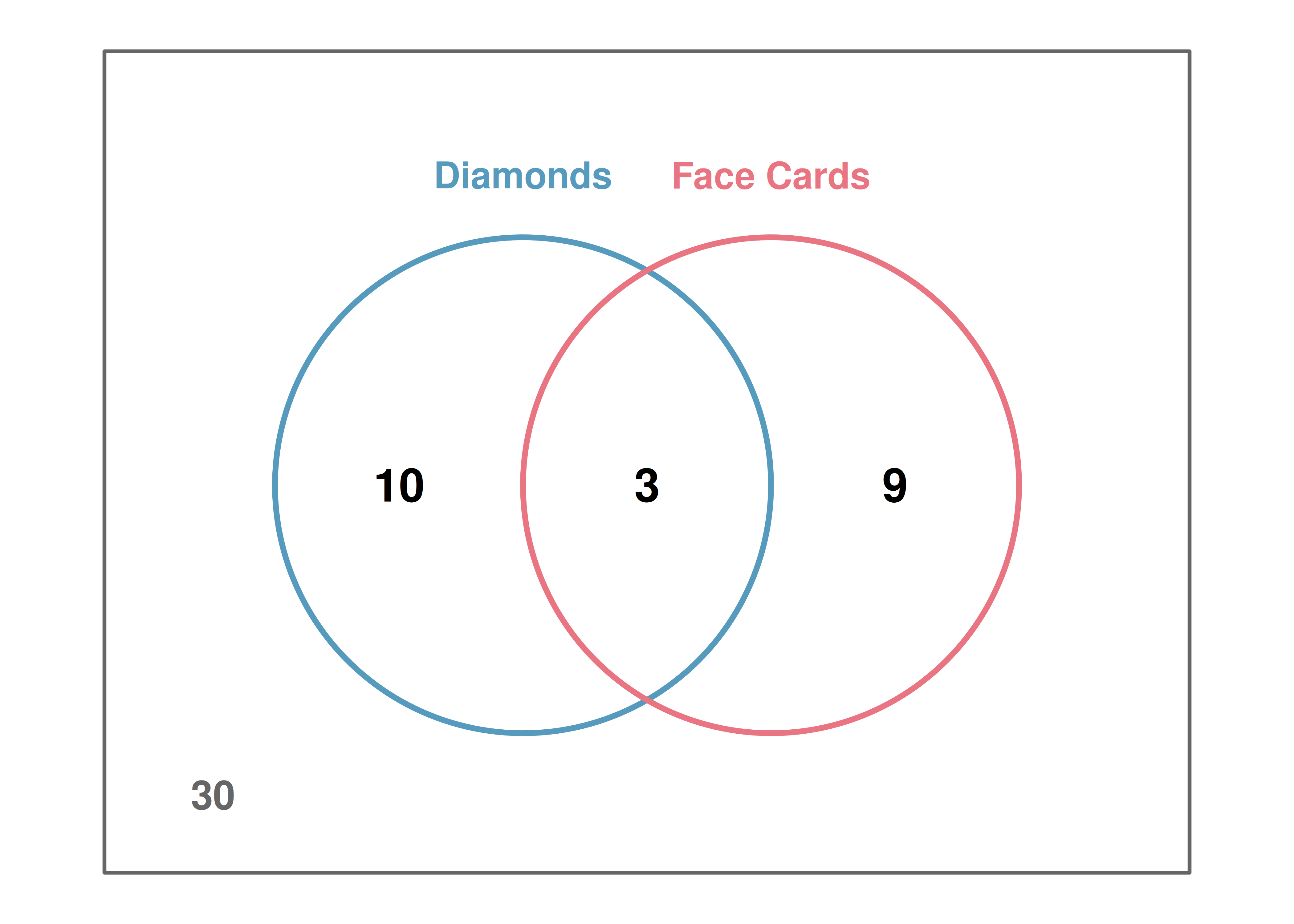
If we compute \(P(A) + P(B) = 13/52 + 12/52 = 25/52\), we have counted the 3 cards in the overlap twice. We correct this:

\[P(A \text{ or } B) = P(A) + P(B) - P(A \text{ and } B) = \frac{13}{52} + \frac{12}{52} - \frac{3}{52} = \frac{22}{52} = \frac{11}{26}\]

General addition rule. For any two events \(A\) and \(B\) (disjoint or not):

\[P(A \text{ or } B) = P(A) + P(B) - P(A \text{ and } B)\]

“Or” is inclusive in statistics. When we write “\(A\) or \(B\),” we mean “\(A\), \(B\), or both” unless explicitly stated otherwise.

1. If \(A\) and \(B\) are disjoint, explain why \(P(A \text{ and } B) = 0\). (b) Show that the general addition rule simplifies to the simpler addition rule when \(A\) and \(B\) are disjoint.

Show answer

1. If \(A\) and \(B\) are disjoint, they can never occur simultaneously, so \(P(A \text{ and } B) = 0\). (b) Substituting 0 for \(P(A \text{ and } B)\) in the general addition rule gives \(P(A \text{ or } B) = P(A) + P(B) - 0 = P(A) + P(B)\), which is the simpler addition rule.

24.5 Conditional probability

24.5.1 Exploring conditional probability with data

There can be rich relationships between two or more variables, and conditional probability provides the framework for exploring them. Suppose we have data from a study classifying 1,822 photos using both a machine learning (ML) algorithm and human judgment:

	Truth: fashion	Truth: not	Total
ML: pred_fashion	197	22	219
ML: pred_not	112	1491	1603
Total	309	1513	1822

If a photo is actually about fashion, what is the chance the ML classifier correctly identified it?

Of the 309 fashion photos, the ML algorithm correctly classified 197:

\[P(\text{ML predicts fashion} \mid \text{truth is fashion}) = \frac{197}{309} = 0.638\]

We call this a conditional probability because we computed the probability under a condition — that the photo was actually about fashion.

24.5.2 Marginal and joint probabilities

A marginal probability is a probability based on a single variable, without regard to other variables. A joint probability is the probability of two or more outcomes occurring together.

From the photo classification data: \(P(\text{ML predicts fashion}) = 219/1822 = 0.120\) is a marginal probability, while \(P(\text{ML predicts fashion and truth is fashion}) = 197/1822 = 0.108\) is a joint probability.

24.5.3 The conditional probability formula

Conditional probability. The conditional probability of outcome \(A\) given condition \(B\) is:

\[P(A \mid B) = \frac{P(A \text{ and } B)}{P(B)}\]

The vertical bar “\(\mid\)” is read as “given.”

Using the photo classification data, we can verify our earlier calculation using proportions alone:

\[P(\text{truth is fashion} \mid \text{ML predicts fashion}) = \frac{P(\text{truth is fashion and ML predicts fashion})}{P(\text{ML predicts fashion})} = \frac{0.108}{0.120} = 0.900\]

If the ML classifier says a photo is about fashion, there is a 90% probability it actually is.

The smallpox dataset provides data on 6,224 individuals in Boston in 1721. Of these, 3.92% were inoculated. Among those not inoculated, 14.11% died. Among those inoculated, only 2.46% died. Write out, in formal notation, the probability a randomly selected person who was not inoculated died from smallpox.

Show answer

\(P(\text{result} = \text{died} \mid \text{inoculated} = \text{no}) = \frac{P(\text{died and not inoculated})}{P(\text{not inoculated})} = \frac{0.1356}{0.9608} = 0.1411\).

24.6 The multiplication rule

24.6.1 Multiplication rule for independent processes

Consider rolling two dice. If \(1/6\) of the time the first die is a 1, and \(1/6\) of those times the second die is also a 1, then:

\[P(\text{both are 1}) = \frac{1}{6} \times \frac{1}{6} = \frac{1}{36}\]

Multiplication rule for independent processes. If \(A\) and \(B\) represent events from two different and independent processes, then:

\[P(A \text{ and } B) = P(A) \times P(B)\]

If there are \(k\) events \(A_1, \ldots, A_k\) from \(k\) independent processes, then:

\[P(A_1 \text{ and } A_2 \text{ and } \cdots \text{ and } A_k) = P(A_1) \times P(A_2) \times \cdots \times P(A_k)\]

About 9% of people are left-handed. Suppose 2 people are selected at random from the US population. (a) What is the probability that both are left-handed? (b) What is the probability that both are right-handed?

Show answer

1. \(0.09 \times 0.09 = 0.0081\). (b) \(P(\text{right-handed}) = 1 - 0.09 = 0.91\), so \(0.91 \times 0.91 = 0.8281\).

Suppose 5 people are selected at random. (a) What is the probability that all are right-handed? (b) What is the probability that not all are right-handed?

Show answer

1. \(0.91^5 = 0.624\). (b) Using the complement: \(P(\text{not all right-handed}) = 1 - 0.624 = 0.376\).

24.6.2 The general multiplication rule

The general multiplication rule handles events that may not be independent:

General multiplication rule. If \(A\) and \(B\) represent two outcomes or events, then:

\[P(A \text{ and } B) = P(A \mid B) \times P(B)\]

This is simply a rearrangement of the conditional probability formula.

In the smallpox data, 96.08% of residents were not inoculated, and 85.88% of those who were not inoculated survived. What is the probability that a resident was not inoculated and lived?

\[P(\text{lived and not inoculated}) = P(\text{lived} \mid \text{not inoculated}) \times P(\text{not inoculated}) = 0.8588 \times 0.9608 = 0.8251\]

24.6.3 Tree diagrams

Tree diagrams are a tool to organize outcomes and probabilities when two or more processes occur in sequence and each process is conditioned on its predecessors.

Suppose 13% of students earned an A on the midterm. Of those who earned an A on the midterm, 47% received an A on the final. Of those who earned lower than an A on the midterm, 11% received an A on the final. You randomly pick up a final exam and notice the student received an A. What is the probability the student also earned an A on the midterm?

We organize the information into a tree diagram:

Figure 24.4: Tree diagram for midterm and final exam grades.

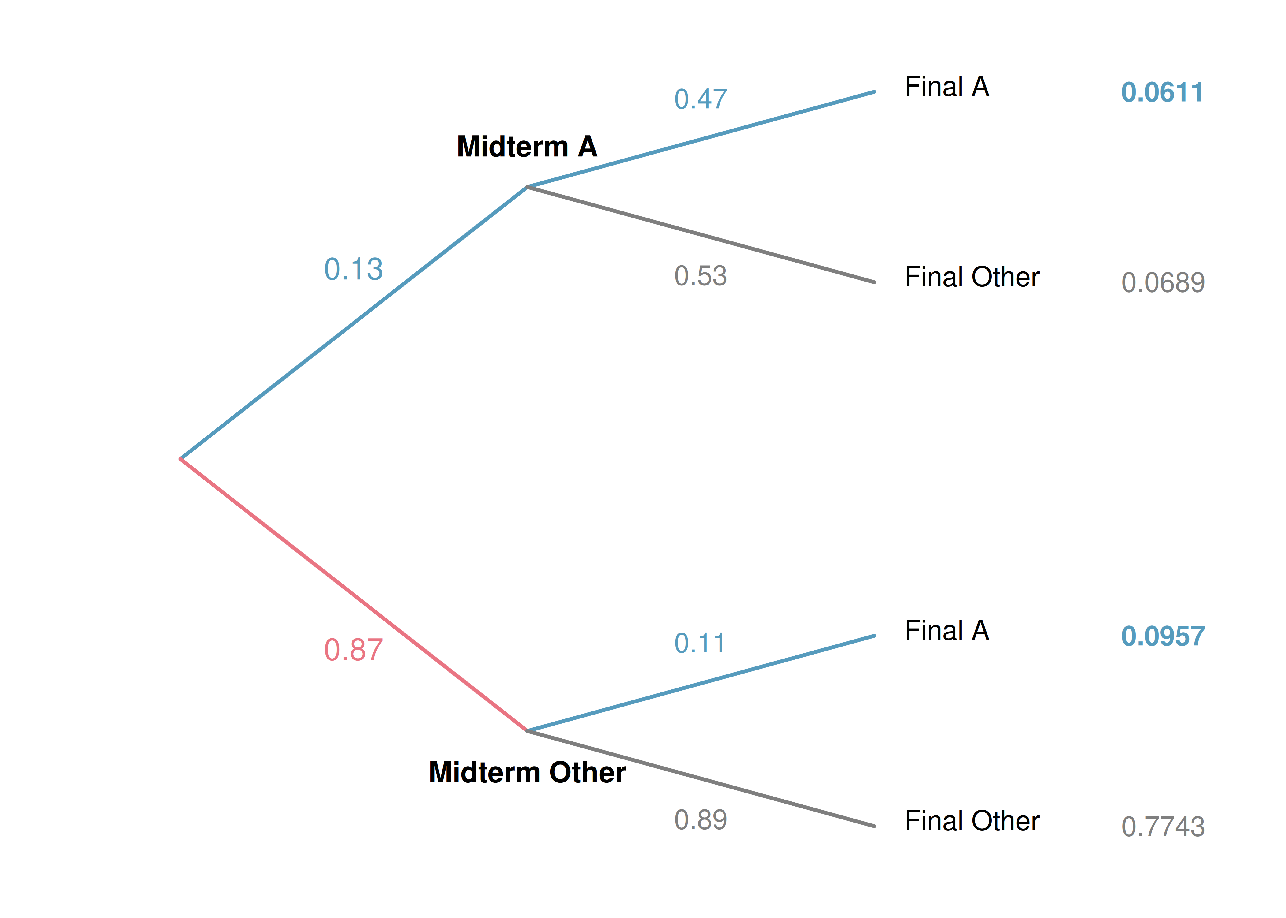
From the tree:

• \(P(\text{midterm A and final A}) = 0.13 \times 0.47 = 0.0611\)
• \(P(\text{final A}) = 0.0611 + 0.0957 = 0.1568\)
• \(P(\text{midterm A} \mid \text{final A}) = \frac{0.0611}{0.1568} = 0.390\)

The probability the student also earned an A on the midterm is about 0.39.

Sum of conditional probabilities. If \(A_1, \ldots, A_k\) represent all disjoint outcomes of a variable, and \(B\) is an event, then:

\[P(A_1 \mid B) + P(A_2 \mid B) + \cdots + P(A_k \mid B) = 1\]

The complement rule also holds for conditional probabilities: \(P(A \mid B) = 1 - P(A^c \mid B)\).

24.7 Independence

Two processes are independent if knowing the outcome of one provides no useful information about the outcome of the other. Mathematically, events \(A\) and \(B\) are independent if:

\[P(A \text{ and } B) = P(A) \times P(B)\]

Equivalently, \(A\) and \(B\) are independent if \(P(A \mid B) = P(A)\).

If we draw one card from a shuffled deck, is the event that the card is a heart independent of the event that the card is an ace?

\(P(\heartsuit) = 1/4\), \(P(\text{ace}) = 1/13\), and \(P(\heartsuit \text{ and ace}) = 1/52\). We check:

\[P(\heartsuit) \times P(\text{ace}) = \frac{1}{4} \times \frac{1}{13} = \frac{1}{52} = P(\heartsuit \text{ and ace})\]

Because the equation holds, “heart” and “ace” are independent events.

Let \(X\) and \(Y\) represent the outcomes of rolling two dice. (a) What is \(P(X = 1)\)? (b) What is \(P(Y = 1 \text{ and } X = 1)\)? (c) Compute \(P(Y = 1 \mid X = 1)\). (d) Compare \(P(Y = 1)\) with the result from (c).

Show answer

1. \(1/6\). (b) \(1/36\). (c) \(\frac{1/36}{1/6} = 1/6\). (d) \(P(Y = 1) = 1/6\), the same as part (c). Knowledge about \(X\) does not change the probability for \(Y\), confirming the dice are independent.

The gambler’s fallacy. Ron is watching a roulette table and notices the last five spins were all black. He bets on red, reasoning that “black six times in a row” is unlikely. This reasoning is flawed: each spin is independent of the previous spins. Past outcomes provide no information about future ones. Casinos often post recent outcomes precisely to encourage this fallacy.

24.8 Bayes’ theorem (optional)

In many situations, we are given \(P(B \mid A)\) but need \(P(A \mid B)\) — the “inverted” conditional probability. Bayes’ theorem provides a systematic way to perform this inversion.

In Canada, about 0.35% of women over 40 develop breast cancer in any given year. Mammograms produce false negatives 11% of the time (indicating no cancer when cancer is present) and false positives 7% of the time (indicating cancer when none is present). If a randomly selected woman over 40 tests positive, what is the probability she actually has breast cancer?

We organize the information into a tree diagram:

Figure 24.5: Tree diagram for breast cancer screening.

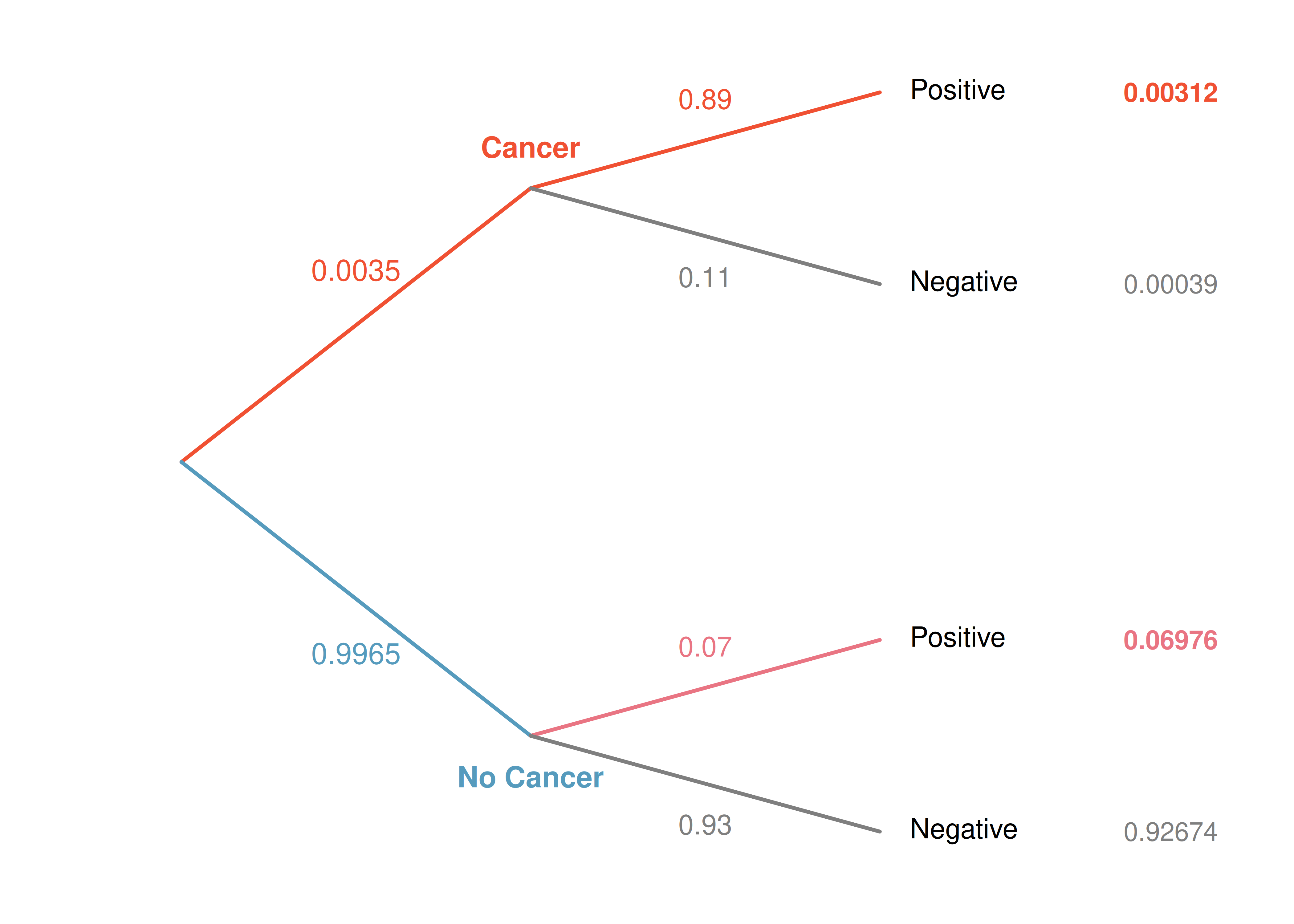
From the tree:

• \(P(\text{cancer and positive}) = 0.0035 \times 0.89 = 0.00312\)
• \(P(\text{positive}) = 0.00312 + 0.06976 = 0.07288\)
• \(P(\text{cancer} \mid \text{positive}) = \frac{0.00312}{0.07288} \approx 0.043\)

Even with a positive mammogram, there is only about a 4% chance the patient has breast cancer. This is why doctors often run additional tests.

Bayes’ theorem. If \(A_1, A_2, \ldots, A_k\) represent all possible disjoint outcomes of a first variable, and \(B\) is an observed outcome of a second variable, then:

\[P(A_1 \mid B) = \frac{P(B \mid A_1) \, P(A_1)}{P(B \mid A_1) \, P(A_1) + P(B \mid A_2) \, P(A_2) + \cdots + P(B \mid A_k) \, P(A_k)}\]

The numerator is the probability of getting both \(A_1\) and \(B\). The denominator is the total (marginal) probability of \(B\).

To apply Bayes’ theorem:

1. Identify the marginal probabilities: \(P(A_1), P(A_2), \ldots, P(A_k)\).
2. Identify the conditional probabilities: \(P(B \mid A_1), P(B \mid A_2), \ldots, P(B \mid A_k)\).
3. Substitute into the formula.

Jose visits campus on Thursday evenings. Academic events occur 35% of evenings, sporting events 20%, and no events 45%. The parking garage fills up 25% of the time during academic events, 70% during sporting events, and 5% when there are no events. If Jose finds the garage full, what is the probability there is a sporting event?

Show answer

Using Bayes’ theorem with \(A_1\) = sporting, \(A_2\) = academic, \(A_3\) = none, and \(B\) = garage full: \(P(\text{sporting} \mid \text{full}) = \frac{0.7 \times 0.2}{0.7 \times 0.2 + 0.25 \times 0.35 + 0.05 \times 0.45} = \frac{0.14}{0.25} = 0.56\). There is a 56% probability of a sporting event.

The strategy of updating beliefs based on new evidence is the foundation of Bayesian statistics, an important branch of statistics that we will not have time to explore further in this course.

24.9 Chapter review

24.9.1 Summary

In this chapter, we developed the mathematical rules of probability:

• Probability is the long-run proportion of times an outcome occurs, governed by the Law of Large Numbers.
• The sample space \(S\) is the set of all possible outcomes; an event is a subset of \(S\).
• Complement rule: \(P(A) = 1 - P(A^c)\).
• Addition rule: \(P(A \text{ or } B) = P(A) + P(B) - P(A \text{ and } B)\). For disjoint events, \(P(A \text{ and } B) = 0\).
• Conditional probability: \(P(A \mid B) = P(A \text{ and } B) / P(B)\).
• Multiplication rule: \(P(A \text{ and } B) = P(A \mid B) \times P(B)\). For independent events, \(P(A \text{ and } B) = P(A) \times P(B)\).
• Events are independent if knowing one occurred does not change the probability of the other.
• Bayes’ theorem inverts conditional probabilities.

24.10 Exercises

1. True or false. For each statement, decide whether it is true or false and explain your reasoning.

1. A basketball player has missed her last 4 free throws (and usually makes about 70%). Her next attempt is therefore more likely to go in than usual.

2. When rolling a fair six-sided die, the events “roll a 4” and “roll an even number” are mutually exclusive.

3. For a given Saturday, \(P(\text{it rains}) + P(\text{it does not rain}) = 1\).

2. Roulette wheel. The game of roulette involves spinning a wheel with 38 slots: 18 red, 18 black, and 2 green. A ball is spun onto the wheel and will eventually land in a slot, where each slot has an equal chance of capturing the ball.

1. You watch a roulette wheel spin 3 consecutive times and the ball lands on a red slot each time. What is the probability that the ball will land on a red slot on the next spin?

2. You watch a roulette wheel spin 300 consecutive times and the ball lands on a red slot each time. What is the probability that the ball will land on a red slot on the next spin?

3. Are you equally confident of your answers to parts (a) and (b)? Why or why not?

3. Four games, one winner. Below are four versions of the same game. Your archnemesis gets to pick the version of the game, and then you get to choose how many times to flip a coin: 10 times or 100 times. Identify how many coin flips you should choose for each version of the game. It costs $1 to play each game. Explain your reasoning.

1. If the proportion of heads is larger than 0.60, you win $1.

2. If the proportion of heads is larger than 0.40, you win $1.

3. If the proportion of heads is between 0.40 and 0.60, you win $1.

4. If the proportion of heads is smaller than 0.30, you win $1.

4. Backgammon. Backgammon is a board game for two players in which the playing pieces are moved according to the roll of two dice. Players win by removing all of their pieces from the board, so it is usually good to roll high numbers. You are playing backgammon with a friend and you roll two 6s in your first roll and two 6s in your second roll. Your friend rolls two 3s in his first roll and again in his second row. Your friend claims that you are cheating, because rolling double 6s twice in a row is very unlikely. Using probability, show that your rolls were just as likely as his.

5. Coin flips. If you flip a fair coin 10 times, what is the probability of

1. getting all tails?

2. getting all heads?

3. getting at least one tails?

6. Dice rolls. If you roll a pair of fair dice, what is the probability of

1. getting a sum of 1?

2. getting a sum of 5?

3. getting a sum of 12?

7. Swing voters. A Pew Research survey asked 2,373 randomly sampled registered voters their political affiliation (Republican, Democrat, or Independent) and whether or not they identify as swing voters. 35% of respondents identified as Independent, 23% identified as swing voters, and 11% identified as both.

1. Are being Independent and being a swing voter disjoint, i.e. mutually exclusive?

2. Draw a Venn diagram summarizing the variables and their associated probabilities.

3. What percent of voters are Independent but not swing voters?

4. What percent of voters are Independent or swing voters?

5. What percent of voters are neither Independent nor swing voters?

6. Is the event that someone is a swing voter independent of the event that someone is a political Independent?

8. Poverty and language. The American Community Survey is an ongoing survey that provides data every year to give communities the current information they need to plan investments and services. The 2010 American Community Survey estimates that 14.6% of Americans live below the poverty line, 20.7% speak a language other than English (foreign language) at home, and 4.2% fall into both categories.

1. Are living below the poverty line and speaking a foreign language at home disjoint?

2. Draw a Venn diagram summarizing the variables and their associated probabilities.

3. What percent of Americans live below the poverty line and only speak English at home?

4. What percent of Americans live below the poverty line or speak a foreign language at home?

5. What percent of Americans live above the poverty line and only speak English at home?

6. Is the event that someone lives below the poverty line independent of the event that the person speaks a foreign language at home?

9. Disjoint vs. independent. In parts (a) and (b), identify whether the events are disjoint, independent, or neither (events cannot be both disjoint and independent).

1. You and a randomly selected student from your class both earn A’s in this course.

2. You and your class study partner both earn A’s in this course.

3. If two events can occur at the same time, must they be dependent?

10. Guessing on an exam. In a multiple choice exam, there are 5 questions and 4 choices for each question (a, b, c, d). Nancy has not studied for the exam at all and decides to randomly guess the answers. What is the probability that:

1. the first question she gets right is the \(5^{th}\) question?

2. she gets all of the questions right?

3. she gets at least one question right?

11. Educational attainment of couples. The table below shows the distribution of education level attained by US residents by gender based on data collected in the 2010 American Community Survey.

c c }		Gender
	9th to 12th grade, no diploma	0.10
Highest	HS graduate (or equivalent)	0.30
education	Some college, no degree	0.22
attained	Associate’s degree	0.06
	Bachelor’s degree	0.16
	Graduate or professional degree	0.09

1. What is the probability that a randomly chosen man has at least a Bachelor’s degree?

2. What is the probability that a randomly chosen woman has at least a Bachelor’s degree?

3. What is the probability that a man and a woman getting married both have at least a Bachelor’s degree? Note any assumptions you must make to answer this question.

4. If you made an assumption in part (c), do you think it was reasonable? If you didn’t make an assumption, double check your earlier answer and then return to this part.

12. School absences. Data collected at elementary schools in DeKalb County, GA suggest that each year roughly 25% of students miss exactly one day of school, 15% miss 2 days, and 28% miss 3 or more days due to sickness.

1. What is the probability that a student chosen at random doesn’t miss any days of school due to sickness this year?

2. What is the probability that a student chosen at random misses no more than one day?

3. What is the probability that a student chosen at random misses at least one day?

4. If a parent has two kids at a DeKalb County elementary school, what is the probability that neither kid will miss any school? Note any assumption you must make to answer this question.

5. If a parent has two kids at a DeKalb County elementary school, what is the probability that both kids will miss some school, i.e. at least one day? Note any assumption you make.

6. If you made an assumption in part (d) or (e), do you think it was reasonable? If you didn’t make any assumptions, double check your earlier answers.

13. Joint and conditional probabilities. P(A) = 0.3, P(B) = 0.7

1. Can you compute P(A and B) if you only know P(A) and P(B)?

2. Assuming that events A and B arise from independent random processes,

3. what is P(A and B)?

4. what is P(A or B)?

5. what is P(A\(|\)B)?

6. If we are given that P(A and B) = 0.1, are the random variables giving rise to events A and B independent?

7. If we are given that P(A and B) = 0.1, what is P(A\(|\)B)?

14. PB & J. Suppose 80% of people like peanut butter, 89% like jelly, and 78% like both. Given that a randomly sampled person likes peanut butter, what’s the probability that he also likes jelly?

15. Global warming. A Pew Research poll asked 1,306 Americans “From what you’ve read and heard, is there solid evidence that the average temperature on earth has been getting warmer over the past few decades, or not?”. The table below shows the distribution of responses by party and ideology, where the counts have been replaced with relative frequencies.

		Response
		warming
Party and	Mod/Lib Republican	0.06
Ideology	Mod/Cons Democrat	0.25
	Liberal Democrat	0.18

1. Are believing that the earth is warming and being a liberal Democrat mutually exclusive?

2. What is the probability that a randomly chosen respondent believes the earth is warming or is a liberal Democrat?

3. What is the probability that a randomly chosen respondent believes the earth is warming given that he is a liberal Democrat?

4. What is the probability that a randomly chosen respondent believes the earth is warming given that he is a conservative Republican?

5. Does it appear that whether or not a respondent believes the earth is warming is independent of their party and ideology? Explain your reasoning.

6. What is the probability that a randomly chosen respondent is a moderate/liberal Republican given that he does not believe that the earth is warming?

16. Health coverage, relative frequencies. The Behavioral Risk Factor Surveillance System (BRFSS) is an annual telephone survey designed to identify risk factors in the adult population and report emerging health trends. The following table displays the distribution of health status of respondents to this survey (excellent, very good, good, fair, poor) and whether or not they have health insurance.

		Health Status
Coverage	Yes	0.2099	0.3123

1. Are being in excellent health and having health coverage mutually exclusive?

2. What is the probability that a randomly chosen individual has excellent health?

3. What is the probability that a randomly chosen individual has excellent health given that he has health coverage?

4. What is the probability that a randomly chosen individual has excellent health given that he doesn’t have health coverage?

5. Do having excellent health and having health coverage appear to be independent?

17. Burger preferences. A 2010 SurveyUSA poll asked 500 Los Angeles residents, “What is the best hamburger place in Southern California? Five Guys Burgers? In-N-Out Burger? Fat Burger? Tommy’s Hamburgers? Umami Burger? Or somewhere else?” The distribution of responses by gender is shown below.

r r r }		Gender
	In-N-Out Burger	162
Best	Fat Burger	10
hamburger	Tommy’s Hamburgers	27
place	Umami Burger	5
	Other	26
	Not Sure	13

1. Are being female and liking Five Guys Burgers mutually exclusive?

2. What is the probability that a randomly chosen male likes In-N-Out the best?

3. What is the probability that a randomly chosen female likes In-N-Out the best?

4. What is the probability that a man and a woman who are dating both like In-N-Out the best? Note any assumption you make and evaluate whether you think that assumption is reasonable.

5. What is the probability that a randomly chosen person likes Umami best or that person is female?

18. Assortative mating. Assortative mating is a nonrandom mating pattern where individuals with similar genotypes and/or phenotypes mate with one another more frequently than what would be expected under a random mating pattern. Researchers studying this topic collected data on eye colors of 204 Scandinavian men and their female partners. The table below summarizes the results.

		Partner (female)
Self (male)	Brown	19
	Green	11

1. What is the probability that a randomly chosen male respondent or his partner has blue eyes?

2. What is the probability that a randomly chosen male respondent with blue eyes has a partner with blue eyes?

3. What is the probability that a randomly chosen male respondent with brown eyes has a partner with blue eyes? What about the probability of a randomly chosen male respondent with green eyes having a partner with blue eyes?

4. Does it appear that the eye colors of male respondents and their partners are independent? Explain your reasoning.

19. Tutoring and passing. A campus tutoring center reports that 70% of statistics students attend tutoring at least once during the semester. Of students who attend, 90% pass the course; of students who don’t attend, 72% pass.

1. Find the probability that a randomly selected student both attends tutoring AND passes.

2. Find the overall probability that a randomly selected student passes.

3. Given that a student passed, find the probability they attended tutoring.

20. Counterfeit detector accuracy. A bank’s automated bill-handling machine scans bills as they are deposited. About 3% of bills it processes are counterfeit. The scanner correctly flags 97% of counterfeit bills as suspicious (its sensitivity), and it has a 5% false-positive rate on genuine bills.

1. What is the overall probability that a randomly chosen bill is flagged as suspicious?

2. Given that a bill is flagged, what is the probability it is actually counterfeit?

3. Explain in one sentence why your answer to (b) is much smaller than the scanner’s sensitivity.

21. It’s never lupus. Lupus is a medical phenomenon where antibodies that are supposed to attack foreign cells to prevent infections instead see plasma proteins as foreign bodies, leading to a high risk of blood clotting. It is believed that 2% of the population suffer from this disease. The test is 98% accurate if a person actually has the disease. The test is 74% accurate if a person does not have the disease. There is a line from the Fox television show House that is often used after a patient tests positive for lupus: “It’s never lupus.” Do you think there is truth to this statement? Use appropriate probabilities to support your answer.

22. Exit poll. Edison Research gathered exit poll results from several sources for the Wisconsin recall election of Scott Walker. They found that 53% of the respondents voted in favor of Scott Walker. Additionally, they estimated that of those who did vote in favor for Scott Walker, 37% had a college degree, while 44% of those who voted against Scott Walker had a college degree. Suppose we randomly sampled a person who participated in the exit poll and found that he had a college degree. What is the probability that he voted in favor of Scott Walker?

23. Marbles in an urn. Imagine you have an urn containing 5 red, 3 blue, and 2 orange marbles in it.

1. What is the probability that the first marble you draw is blue?

2. Suppose you drew a blue marble in the first draw. If drawing with replacement, what is the probability of drawing a blue marble in the second draw?

3. Suppose you instead drew an orange marble in the first draw. If drawing with replacement, what is the probability of drawing a blue marble in the second draw?

4. If drawing with replacement, what is the probability of drawing two blue marbles in a row?

5. When drawing with replacement, are the draws independent? Explain.

24. Socks in a drawer. In your sock drawer you have 4 blue, 5 gray, and 3 black socks. Half asleep one morning you grab 2 socks at random and put them on. Find the probability you end up wearing

1. 2 blue socks

2. no gray socks

3. at least 1 black sock

4. a green sock

5. matching socks

25. Chips in a bag. Imagine you have a bag containing 5 red, 3 blue, and 2 orange chips.

1. Suppose you draw a chip and it is blue. If drawing without replacement, what is the probability the next is also blue?

2. Suppose you draw a chip and it is orange, and then you draw a second chip without replacement. What is the probability this second chip is blue?

3. If drawing without replacement, what is the probability of drawing two blue chips in a row?

4. When drawing without replacement, are the draws independent? Explain.

26. Books on a bookshelf. The table below shows the distribution of books on a bookcase based on whether they are nonfiction or fiction and hardcover or paperback.

		Format
	Nonfiction	15

1. Find the probability of drawing a hardcover book first then a paperback fiction book second when drawing without replacement.

2. Determine the probability of drawing a fiction book first and then a hardcover book second, when drawing without replacement.

3. Calculate the probability of the scenario in part (b), except this time complete the calculations under the scenario where the first book is placed back on the bookcase before randomly drawing the second book.

4. The final answers to parts (b) and (c) are very similar. Explain why this is the case.

27. Student outfits. In a classroom with 24 students, 7 students are wearing jeans, 4 are wearing shorts, 8 are wearing skirts, and the rest are wearing leggings. If we randomly select 3 students without replacement, what is the probability that one of the selected students is wearing leggings and the other two are wearing jeans? Note that these are mutually exclusive clothing options.

28. The birthday problem. Suppose we pick three people at random. For each of the following questions, ignore the special case where someone might be born on February 29th, and assume that births are evenly distributed throughout the year.

1. What is the probability that the first two people share a birthday?

2. What is the probability that at least two people share a birthday?

29. Health coverage, frequencies. The Behavioral Risk Factor Surveillance System (BRFSS) is an annual telephone survey designed to identify risk factors in the adult population and report emerging health trends. The following table summarizes two variables for the respondents: health status and health coverage, which describes whether each respondent had health insurance.

		Health Status
Coverage	Yes	4,198	6,245

1. If we draw one individual at random, what is the probability that the respondent has excellent health and doesn’t have health coverage?

2. If we draw one individual at random, what is the probability that the respondent has excellent health or doesn’t have health coverage?

30. HIV in Swaziland. Swaziland has the highest HIV prevalence in the world: 25.9% of this country’s population is infected with HIV. The ELISA test is one of the first and most accurate tests for HIV. For those who carry HIV, the ELISA test is 99.7% accurate. For those who do not carry HIV, the test is 92.6% accurate. If an individual from Swaziland has tested positive, what is the probability that he carries HIV?

31. Defective sample from one machine. A factory produces parts on two machines. Machine A makes 40% of the output and has a 2% defect rate; Machine B makes the remaining 60% with a 5% defect rate. You take three parts from the same (unknown) machine and find that all three are defective.

1. Given that all three parts are defective, what is the probability they came from Machine A?

2. Why is the answer in (a) much smaller than the prior probability that a randomly chosen machine is Machine A?