27 Binomial Distribution

How many of 400 randomly sampled adults are left-handed? How many of 20 randomly selected parts from an assembly line are defective? These “count of successes” questions arise constantly in statistics and are answered by the binomial distribution. In this chapter, we identify the four conditions that define a binomial setting, develop the formula for computing binomial probabilities, derive the mean and standard deviation, and show how the normal distribution can approximate binomial probabilities when the sample size is large.

27.1 The binomial setting

The binomial distribution describes the number of successes in a fixed number of independent trials, where each trial has only two possible outcomes.

The four binomial conditions. A random variable $X$ follows a binomial distribution if:

Fixed number of trials: The number of trials $n$ is fixed in advance.
Binary outcomes: Each trial results in one of two outcomes, which we label “success” and “failure.”
Independence: The trials are independent — the outcome of one trial does not affect the outcome of any other trial.
Constant probability: The probability of success $p$ is the same for every trial.

If all four conditions are met, we say $X$ follows a binomial distribution with parameters $n$ and $p$, written $X \sim \text{Binomial}(n, p)$.

A health insurance company found that 70% of the people they insure stay below their deductible in any given year. Consider a random sample of four individuals. Does the number who stay below their deductible follow a binomial distribution?

Fixed $n$: Yes, $n = 4$ individuals.
Binary: Yes, each person either stays below the deductible (success) or exceeds it (failure).
Independence: Yes, because the sample is random from a large population.
Constant $p$: Yes, each person has a 70% chance of staying below the deductible.

All four conditions are met, so $X \sim \text{Binomial}(n = 4, p = 0.70)$.

The labels “success” and “failure” are just conventions — a “success” does not have to be a good outcome. If we are counting defective parts, a “success” might be finding a defective part. The mathematical framework does not depend on which outcome we call a success, as long as we are consistent.

The probability that a random smoker will develop a severe lung condition is about 0.3. If you have 4 friends who smoke, are the conditions for the binomial model satisfied?

Show answer

This is questionable. If the friends know each other, the independence condition may be violated. Acquaintances may have similar smoking habits or might influence each other. If, however, we could treat them as a random sample of smokers, the conditions would be approximately met.

27.1.1 The Bernoulli distribution: a single trial

A single trial with two outcomes is called a Bernoulli trial, and the resulting random variable is a Bernoulli random variable.

If $X$ is a random variable that takes value 1 with probability $p$ (success) and 0 with probability $1 - p$ (failure), then $X$ is a Bernoulli random variable with:

\[\mu = p \qquad \sigma = \sqrt{p(1-p)}\]

A binomial random variable is simply the sum of $n$ independent Bernoulli random variables, each with the same probability $p$.

27.2 Computing binomial probabilities

27.2.1 Building the formula

Let’s find the probability that exactly 1 of 4 randomly selected insured individuals exceeds the deductible (so 3 “successes” — staying below — and 1 “failure”).

Consider the specific scenario where person A exceeds and persons B, C, D do not:

\[P(A = \text{exceed}, B = \text{not}, C = \text{not}, D = \text{not}) = (0.3)(0.7)(0.7)(0.7) = (0.7)^3(0.3)^1 = 0.103\]

But there are four such scenarios — any one of the four people could be the one who exceeds. Each scenario has the same probability. So:

\[P(\text{exactly 3 successes in 4 trials}) = 4 \times (0.7)^3(0.3)^1 = 0.412\]

The general pattern is:

\[P(X = k) = [\text{number of arrangements}] \times [\text{probability of one arrangement}]\]

27.2.2 The binomial coefficient

The number of ways to arrange $k$ successes in $n$ trials is given by the binomial coefficient:

\[\binom{n}{k} = \frac{n!}{k!(n-k)!}\]

read as “$n$ choose $k$,” where $n!$ (read “$n$ factorial”) means $n \times (n-1) \times \cdots \times 2 \times 1$, with the special case $0! = 1$.

For our example: $\binom{4}{3} = \frac{4!}{3! \cdot 1!} = \frac{24}{6 \times 1} = 4$, confirming the four arrangements we identified.

27.2.3 The binomial probability formula

Binomial probability formula. If $X \sim \text{Binomial}(n, p)$, the probability of exactly $k$ successes is:

\[P(X = k) = \binom{n}{k} p^k (1-p)^{n-k} = \frac{n!}{k!(n-k)!} \, p^k (1-p)^{n-k}\]

for $k = 0, 1, 2, \ldots, n$.

What is the probability that 5 of 8 randomly selected insured individuals will not exceed the deductible?

With $n = 8$, $k = 5$, and $p = 0.70$:

\[P(X = 5) = \binom{8}{5}(0.70)^5(0.30)^3\]

Computing the binomial coefficient:

\[\binom{8}{5} = \frac{8!}{5! \cdot 3!} = \frac{8 \times 7 \times 6}{3 \times 2 \times 1} = 56\]

And the probability of a single arrangement: $(0.70)^5(0.30)^3 \approx 0.00454$.

\[P(X = 5) = 56 \times 0.00454 \approx 0.254\]

Suppose 4 friends who smoke can be treated as a random sample, with $P(\text{severe lung condition}) = 0.3$ for each. (a) What is the probability that none develop a severe lung condition? (b) What is the probability that exactly one does? (c) What is the probability that at most one does?

Show answer

$P(X = 0) = \binom{4}{0}(0.3)^0(0.7)^4 = 1 \times 1 \times 0.2401 = 0.2401$. (b) $P(X = 1) = \binom{4}{1}(0.3)^1(0.7)^3 = 4 \times 0.3 \times 0.343 = 0.4116$. (c) $P(X \leq 1) = P(X = 0) + P(X = 1) = 0.2401 + 0.4116 = 0.6517$.

What is the probability that at least 2 of the 4 smoking friends will develop a severe lung condition?

Show answer

Using the complement: $P(X \geq 2) = 1 - P(X \leq 1) = 1 - 0.6517 = 0.3483$.

27.2.4 Computing binomial probabilities in practice

For small values of $n$ and $k$, the binomial formula can be computed by hand. For larger problems, use technology:

StatLens: The Binomial Distribution calculator computes probabilities and visualizes the distribution.
Calculator: Most graphing calculators have a binompdf and binomcdf function.
Software: Any statistical software can compute binomial probabilities. Look for functions named something like “binomial CDF” or “binomial probability.”

For example, to find $P(X \leq 42)$ when $X \sim \text{Binomial}(400, 0.15)$, computing 43 individual probabilities by hand would be impractical. Using the StatLens Binomial calculator with $n = 400$, $p = 0.15$, and $P(X \leq 42)$, we get approximately 0.0054.

27.3 Mean and standard deviation

Mean and standard deviation of a binomial distribution. If $X \sim \text{Binomial}(n, p)$, then:

\[\mu = np \qquad \sigma = \sqrt{np(1-p)}\]

These formulas follow from the fact that a binomial random variable is the sum of $n$ independent Bernoulli random variables, each with mean $p$ and variance $p(1-p)$.

If 40 individuals are randomly sampled and each has a 70% chance of staying below their insurance deductible, how many would you expect to stay below? What is the standard deviation?

\[\mu = np = 40 \times 0.70 = 28\]

\[\sigma = \sqrt{np(1-p)} = \sqrt{40 \times 0.70 \times 0.30} = \sqrt{8.4} \approx 2.9\]

We expect about 28 individuals to stay below their deductible, give or take about 2.9. Using the rough “95% within 2 standard deviations” guideline, we would expect between about 22 and 34 individuals in most samples.

Suppose 7 friends who smoke can be treated as a random sample, with $p = 0.3$ for developing a severe lung condition. How many would you expect to develop the condition? What is the standard deviation?

Show answer

$\mu = np = 7 \times 0.3 = 2.1$. $\sigma = \sqrt{7 \times 0.3 \times 0.7} = \sqrt{1.47} \approx 1.21$. You would expect about 2 of the 7 friends to develop a severe lung condition.

27.3.1 Simulation perspective: Does the formula match reality?

We can verify the binomial formulas using simulation. Consider $X \sim \text{Binomial}(n = 20, p = 0.3)$:

Theory: $\mu = 20 \times 0.3 = 6$ and $\sigma = \sqrt{20 \times 0.3 \times 0.7} = \sqrt{4.2} \approx 2.05$
Simulation: Generate 10,000 binomial random samples, each with $n = 20$ and $p = 0.3$. The sample mean of the 10,000 counts will be very close to 6, and the sample standard deviation will be very close to 2.05.

This is another instance of the Law of Large Numbers: the simulated distribution converges to the theoretical distribution as we increase the number of simulations.

See it in action. Open the Binomial Distribution Explorer, set $n = 20$ and $p = 0.3$, then simulate 1,000 experiments and watch the histogram converge to the theoretical distribution.

27.4 Normal approximation to the binomial

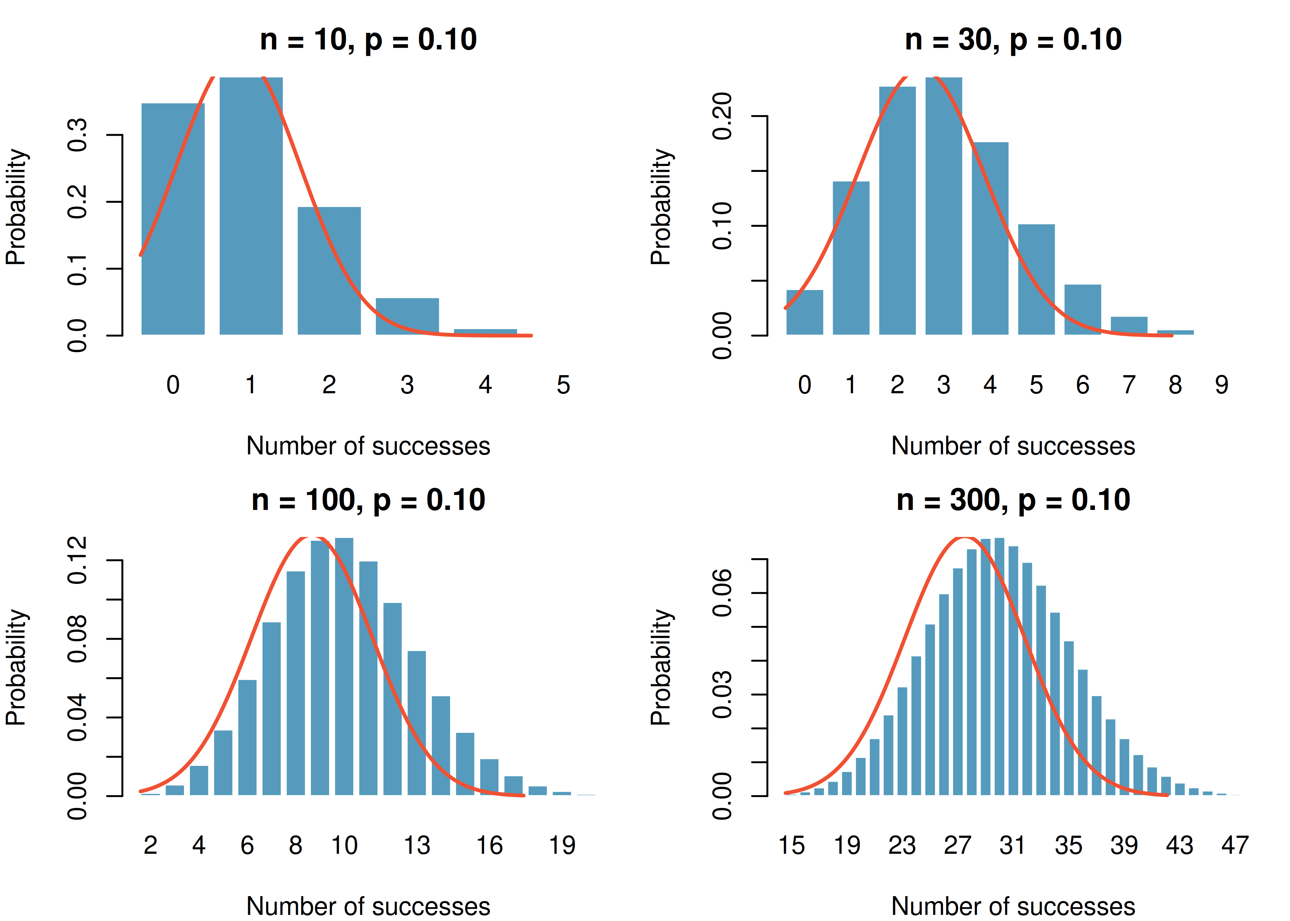
The binomial formula can be cumbersome for large $n$, especially when computing cumulative probabilities like $P(X \leq 42)$ for $n = 400$. Fortunately, when $n$ is large enough, the binomial distribution is well approximated by the normal distribution.

Approximately 15% of the US population smokes cigarettes. A local government surveyed 400 randomly selected individuals and found only 42 smokers. If the true proportion is 0.15, what is the probability of observing 42 or fewer smokers?

The exact answer requires summing 43 binomial probabilities, which gives $P(X \leq 42) = 0.0054$.

As the sample size increases, the binomial distribution becomes increasingly bell-shaped and symmetric. This is illustrated in the figure below.

Four histograms of binomial distributions with p = 0.10. For n = 10, the distribution is right-skewed. For n = 30, it is slightly skewed. For n = 100 and n = 300, the distribution is approximately symmetric and bell-shaped. — Figure 27.1: Binomial distributions with p = 0.10 and sample sizes n = 10, 30, 100, and 300. As n increases, the distribution approaches a normal curve. ↗ Try this live — drive $n$ and $p$ in the Binomial PMF and watch the shape settle.

Normal approximation to the binomial. The binomial distribution with parameters $n$ and $p$ is approximately normal when both $np \geq 10$ and $n(1-p) \geq 10$. The approximating normal distribution has:

\[\mu = np \qquad \sigma = \sqrt{np(1-p)}\]

Use the normal approximation to estimate $P(X \leq 42)$ for $X \sim \text{Binomial}(400, 0.15)$.

First, check the conditions: $np = 400 \times 0.15 = 60 \geq 10$ and $n(1-p) = 400 \times 0.85 = 340 \geq 10$. The normal approximation is appropriate.

The approximating distribution is $N(\mu = 60, \sigma = 7.14)$, where $\sigma = \sqrt{400 \times 0.15 \times 0.85} = 7.14$.

Compute the Z-score:

\[Z = \frac{42 - 60}{7.14} = \frac{-18}{7.14} = -2.52\]

Using the standard normal distribution: $P(Z \leq -2.52) = 0.0059$.

This is very close to the exact binomial probability of 0.0054.

A coin is flipped 100 times. Use the normal approximation to find the probability of getting 60 or more heads.

Show answer

Check conditions: $np = 100 \times 0.5 = 50 \geq 10$ and $n(1-p) = 50 \geq 10$. The approximation is appropriate. $\mu = 50$, $\sigma = \sqrt{100 \times 0.5 \times 0.5} = 5$. $Z = (60 - 50)/5 = 2$. $P(Z \geq 2) = 1 - 0.9772 = 0.0228$. There is about a 2.3% chance of getting 60 or more heads in 100 flips of a fair coin.

27.4.1 Connecting to inference

The normal approximation to the binomial is not just a computational shortcut — it is the theoretical basis for the inference methods we developed in Parts II and III. When we studied the sampling distribution of the sample proportion $\hat{p}$ in the sampling distributions chapter, we were implicitly using the fact that the count of successes $X$ in a sample of size $n$ follows a binomial distribution, and that this binomial distribution is approximately normal for large $n$.

Specifically, if $X \sim \text{Binomial}(n, p)$, then $\hat{p} = X/n$, and the normal approximation tells us:

\[\hat{p} \approx N\left(p, \sqrt{\frac{p(1-p)}{n}}\right)\]

This is exactly the result we used when constructing confidence intervals and performing hypothesis tests for proportions in the inference for proportions chapter. The theory developed in this chapter explains why those methods work.

27.5 Chapter review

27.5.1 Summary

The binomial distribution counts the number of successes in $n$ independent trials, each with the same probability of success $p$.
Four conditions: fixed $n$, binary outcomes, independence, constant $p$.
Binomial probability formula: $P(X = k) = \binom{n}{k} p^k (1-p)^{n-k}$
Mean and standard deviation: $\mu = np$ and $\sigma = \sqrt{np(1-p)}$.
When $np \geq 10$ and $n(1-p) \geq 10$, the binomial distribution is well approximated by the normal distribution $N(np, \sqrt{np(1-p)})$.
The normal approximation to the binomial provides the theoretical justification for the inference methods on proportions from the inference for proportions chapter.

27.6 Exercises

Underage drinking, Part I. Data collected by the Substance Abuse and Mental Health Services Administration (SAMSHA) suggests that 69.7% of 18-20 year olds consumed alcoholic beverages in any given year.

Suppose a random sample of ten 18-20 year olds is taken. Is the use of the binomial distribution appropriate for calculating the probability that exactly six consumed alcoholic beverages? Explain.
Calculate the probability that exactly 6 out of 10 randomly sampled 18- 20 year olds consumed an alcoholic drink.
What is the probability that exactly four out of ten 18-20 year olds have not consumed an alcoholic beverage?
What is the probability that at most 2 out of 5 randomly sampled 18-20 year olds have consumed alcoholic beverages?
What is the probability that at least 1 out of 5 randomly sampled 18-20 year olds have consumed alcoholic beverages?

Chickenpox, Part I. Boston Children’s Hospital estimates that 90% of Americans have had chickenpox by the time they reach adulthood.

Suppose we take a random sample of 100 American adults. Is the use of the binomial distribution appropriate for calculating the probability that exactly 97 out of 100 randomly sampled American adults had chickenpox during childhood? Explain.
Calculate the probability that exactly 97 out of 100 randomly sampled American adults had chickenpox during childhood.
What is the probability that exactly 3 out of a new sample of 100 American adults have not had chickenpox in their childhood?
What is the probability that at least 1 out of 10 randomly sampled American adults have had chickenpox?
What is the probability that at most 3 out of 10 randomly sampled American adults have not had chickenpox?

Underage drinking, Part II. We learned in a previous exercise that about 70% of 18-20 year olds consumed alcoholic beverages in any given year. We now consider a random sample of fifty 18-20 year olds.

How many people would you expect to have consumed alcoholic beverages? And with what standard deviation?
Would you be surprised if there were 45 or more people who have consumed alcoholic beverages?
What is the probability that 45 or more people in this sample have consumed alcoholic beverages? How does this probability relate to your answer to part (b)?

Chickenpox, Part II. We learned in a previous exercise that about 90% of American adults had chickenpox before adulthood. We now consider a random sample of 120 American adults.

How many people in this sample would you expect to have had chickenpox in their childhood? And with what standard deviation?
Would you be surprised if there were 105 people who have had chickenpox in their childhood?
What is the probability that 105 or fewer people in this sample have had chickenpox in their childhood? How does this probability relate to your answer to part (b)?

Four-color spinner. A carnival booth has a four-color spinner divided into four equal sectors: red, blue, green, and yellow. You spin the wheel three times. Each spin is independent and each color has probability $1/4$ per spin. Calculate the probability of getting

at least one red in 3 spins.
exactly 2 reds.
exactly 1 blue.
at most 2 greens.

Arachnophobia. A Gallup Poll found that 7% of teenagers (ages 13 to 17) suffer from arachnophobia and are extremely afraid of spiders. At a summer camp there are 10 teenagers sleeping in each tent. Assume that these 10 teenagers are independent of each other.%

Calculate the probability that at least one of them suffers from arachnophobia.
Calculate the probability that exactly 2 of them suffer from arachnophobia.
Calculate the probability that at most 1 of them suffers from arachnophobia.
If the camp counselor wants to make sure no more than 1 teenager in each tent is afraid of spiders, does it seem reasonable for him to randomly assign teenagers to tents?

Eye color, Part II. a previous exercise introduces a husband and wife with brown eyes who have 0.75 probability of having children with brown eyes, 0.125 probability of having children with blue eyes, and 0.125 probability of having children with green eyes.

What is the probability that their first child will have green eyes and the second will not?
What is the probability that exactly one of their two children will have green eyes?
If they have six children, what is the probability that exactly two will have green eyes?
If they have six children, what is the probability that at least one will have green eyes?
What is the probability that the first green eyed child will be the $4^{th}$ child?
Would it be considered unusual if only 2 out of their 6 children had brown eyes?

Sickle cell anemia. Sickle cell anemia is a genetic blood disorder where red blood cells lose their flexibility and assume an abnormal, rigid, “sickle” shape, which results in a risk of various complications. If both parents are carriers of the disease, then a child has a 25% chance of having the disease, 50% chance of being a carrier, and 25% chance of neither having the disease nor being a carrier. If two parents who are carriers of the disease have 3 children, what is the probability that

two will have the disease?
none will have the disease?
at least one will neither have the disease nor be a carrier?
the first child with the disease will the be $3^{rd}$ child?

Playlist orderings. A music app has 8 different songs in a playlist and plays them in a random order with no repeats — every distinct ordering is equally likely.

How many distinct orderings of the 8 songs are possible?
What is the probability that “Track 1” is played first?
What is the probability that “Track 1” is played first AND “Track 2” is played last?

Allergic campers in a cabin. At a summer camp, cabins hold 4 campers. Independently for each camper, the probability of being allergic to a particular plant is 0.15.

The orderings of (A = allergic, N = not allergic) for a cabin of 4 that have exactly 2 allergic campers are: AANN, ANAN, ANNA, NAAN, NANA, NNAA. How many distinct orderings is that?
Compute the probability of one specific ordering with exactly 2 allergic campers (for example, AANN).
Use the binomial formula to compute the probability that exactly 2 of the 4 campers are allergic.
Multiplying your answers from (a) and (b) should give the answer to (c). Explain why this works.

Airline overbooking. A regional airline runs flights on a small commuter plane with 50 seats. Historically, 7% of booked passengers do not show up, so the airline sells 54 tickets for each flight. Let $X$ be the number of ticketed passengers who actually show up, modeled as $X \sim \text{Binomial}(n = 54, p = 0.93)$.

Find the mean $\mu$ of $X$.
Find the standard deviation $\sigma$ of $X$.
Using the normal approximation with continuity correction, estimate the probability the flight is overbooked, $P(X > 50)$.
Interpret your answer to part (c) in plain language.

Email campaign opens. A marketing team sends a promotional email to 8,000 independent recipients. Historically, each recipient opens the email with probability 0.12, and opens are independent. Let $X$ be the number of recipients who open the email, so $X \sim \text{Binomial}(n = 8000, p = 0.12)$. The team wants the probability that at least 1,000 recipients open the email.

Compute $\mu = E(X)$ and $\sigma = \text{SD}(X)$.
Using the normal approximation with continuity correction, find the z-score corresponding to “at least 1,000 opens.”
Approximate $P(X \ge 1000)$.
State the condition that makes the normal approximation appropriate here.

StatLens Exercises

Let StatLens do the arithmetic; spend your effort on the reasoning a calculator can’t do.

Does this scenario fit the binomial? The binomial requires (i) a fixed number of trials $n$, (ii) two outcomes per trial, (iii) constant success probability $p$, and (iv) independence across trials. For each scenario, check the four conditions and decide whether the binomial applies.
1. Flip a fair coin 50 times; count the number of heads.
2. Draw 5 cards without replacement from a deck; count the number of aces.
3. Survey 100 randomly selected adults; count how many own a smartphone.
4. Roll a die until you get the first 6; count the number of rolls.
5. Test 200 light bulbs from one production line; count how many fail within 100 hours.
Read the binomial PMF. Open the Binomial tool. Set $n = 20$ and $p = 0.3$.
1. Report $P(X = 6)$ (the bar at $X = 6$). Where is the mode of the distribution?
2. Compute the mean and standard deviation from the formulas $\mu = np$ and $\sigma = \sqrt{np(1-p)}$. How close is the visible “center” of the bars to your computed $\mu$?
3. Switch to cumulative mode. What is $P(X \le 5)$? What is $P(X \ge 8)$?
4. Toggle on the normal approximation overlay. Does it match the binomial bars well at $n = 20$, $p = 0.3$? Why or why not?
The normal approximation to the binomial — when does it work? Still in the Binomial tool.
1. Set $n = 20$, $p = 0.05$ (rare event). What does the PMF look like — symmetric or skewed? Turn on the normal overlay. Does the normal model fit?
2. Now $n = 200$, $p = 0.05$. PMF shape? Normal fit?
3. State the success–failure rule: the normal approximation works well when $np \ge 10$ and $n(1-p) \ge 10$. Check this for cases (a) and (b).
4. Why does the rule use both $np \ge 10$ and $n(1-p) \ge 10$ rather than just one? (Hint: consider $p = 0.99$, $n = 100$.)
Connecting the binomial to one-proportion inference. A study of 200 randomly chosen tablet users finds 14 who experienced a side effect, $\hat{p} = 14/200 = 0.07$.
1. Under $H_0: p = 0.10$, the count $X$ of side effects is $X \sim \text{Binomial}(200, 0.10)$. Use the Binomial tool in cumulative mode to find the exact $P(X \le 14)$.
2. Now use the One-Proportion $z$-Test tool with this scenario, $H_A: p < 0.10$. Report the (normal-approximation) p-value. How close is it to the binomial’s exact answer in (a)?
3. Check the success–failure condition under $H_0$. Should you trust the $z$-test’s p-value?
4. In one sentence, when would you prefer the exact binomial probability over the approximate $z$-test p-value?
Expectation and the law of large numbers. A casino offers a game with $n = 100$ trials, win probability $p = 0.45$ per trial, and a $\$1$ wager per trial.
1. Open Binomial $n = 100, p = 0.45$. What’s the expected number of wins? What’s the probability you come out ahead (more than 50 wins)?
2. Now consider playing 100 rounds of this game (100 sessions of 100 trials each). What does the law of large numbers predict about your average per-round winnings as the number of rounds grows?
3. A player says: “In each round my expected loss is small ($-\$10$), so I should keep playing.” Why is this the gambler’s mathematical mistake (not just a sentiment)?
4. How does the binomial probability of “coming out ahead” change as $n$ grows from 100 to 1000 to 10000 trials? Why?