9  Bootstrap Confidence Intervals

In the sampling variability chapter, we saw that sample statistics vary from sample to sample. This variability is not a nuisance — it’s the key to quantifying uncertainty. In this chapter, we learn bootstrapping: a simulation-based method for constructing confidence intervals that requires no formulas and no assumptions about the shape of the population.

9.1 The big idea: resampling

In 2011, researchers collected a sample of 648 pennies in circulation and recorded how old each penny was (current year minus year minted). The question: what is the average age of all pennies currently in circulation in the United States?

The sample mean is \(\bar{x} = 10.4\) years. This is our point estimate of the population mean \(\mu\). But how precise is this estimate? If we collected a different sample of 648 pennies, we’d get a different \(\bar{x}\). We can’t keep collecting new samples — we only have this one.

The bootstrap idea: Treat your sample as a stand-in for the population and resample from it. Each bootstrap resample is drawn with replacement from your original sample, at the same sample size \(n\).

A bootstrap resample is a sample of size \(n\) drawn with replacement from the original sample. The statistic computed from a bootstrap resample is called a bootstrap statistic. The collection of many bootstrap statistics forms the bootstrap distribution.

Why does resampling from our own sample work? If the original sample is representative of the population, then resampling from it mimics what would happen if we could repeatedly sample from the population itself. The variability we see in the bootstrap distribution approximates the true sampling variability of our statistic.

9.2 Bootstrapping a sample mean

Let’s build a bootstrap confidence interval step by step.

9.2.1 Step 1: Collect data

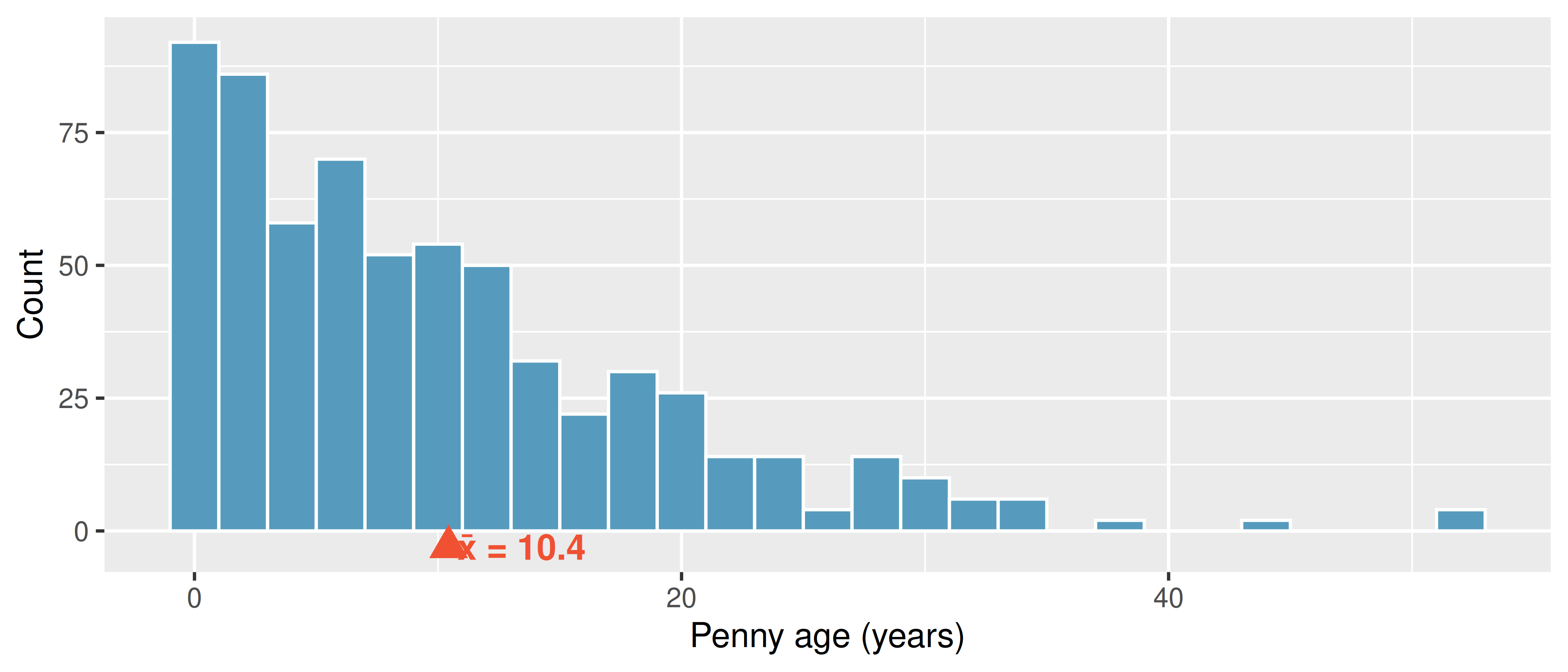
Our sample of 648 pennies has a right-skewed distribution — many young pennies and a long tail of older ones:

Figure 9.1: Distribution of ages for 648 pennies sampled from circulation. The distribution is right-skewed with a mean of about 10.4 years. The sample mean is marked with a red triangle. Open in StatLens

The sample mean is \(\bar{x} = 10.4\) years. Notice the distribution is clearly not bell-shaped — it’s skewed right. Bootstrapping doesn’t care. It works regardless of the population shape.

9.2.2 Step 2: Resample with replacement

We draw a new sample of 648 values from the original 648, with replacement. Some pennies will appear more than once; others will be left out. Each such draw is one bootstrap resample, and the mean of that resample is a bootstrap statistic \(\bar{x}^*\).

9.2.3 Step 3: Repeat many times

We repeat Step 2 a large number of times — typically \(B = 1{,}000\) or more — and record the bootstrap mean \(\bar{x}^*\) each time. This gives us a bootstrap distribution.

Figure 9.2: Building up the bootstrap distribution. With 10 resamples we see only a rough sketch; by 1,000 resamples the shape of the distribution is clear — and approximately bell-shaped (normal), even though the original data are skewed. Open in StatLens

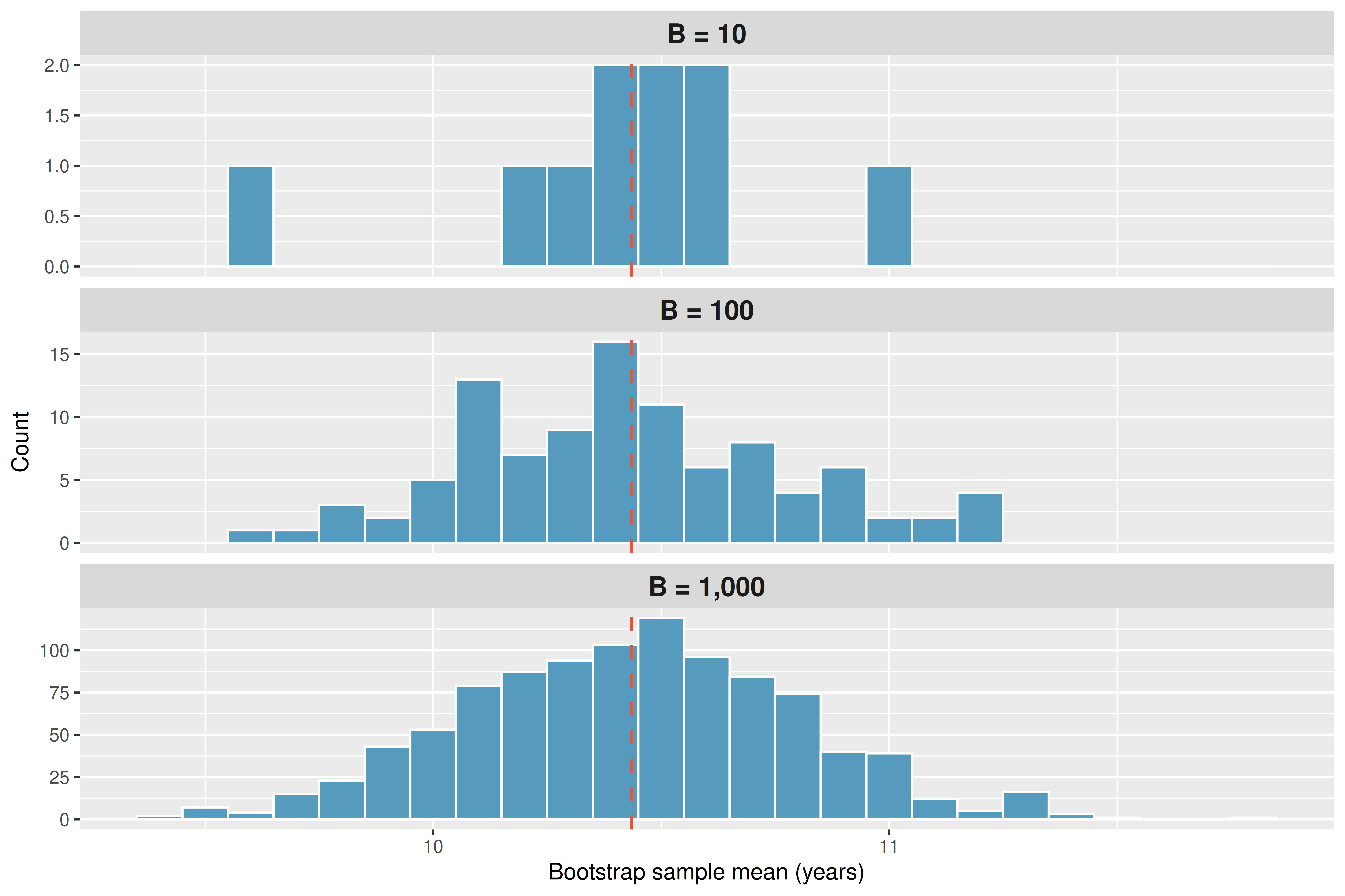
Notice two things: (1) the bootstrap distribution is centered near the original sample mean (dashed red line), and (2) even though the penny ages are right-skewed, the bootstrap distribution of the mean is approximately bell-shaped (what statisticians call a normal shape — recall this term from the empirical rule in Section 4.7). This is the Central Limit Theorem at work — we’ll explore it more in the next chapter.

Predict → Do → Explain. Open the Bootstrap Resampling Activity — the gated activity opens with a Predict step (commit to the bootstrap distribution’s center, spread, and shape before the buildup starts), walks you through generating 1, 10, 100, and 1,000 resamples in sequence with a reality-check gate at each stage, and closes with an Explain step where you articulate why the bootstrap distribution centers where it does and why it looks bell-shaped even when the raw data are skewed. Your predictions and explanation save locally in the tool, so you can leave the activity and return to your work on the same device.

9.2.4 Step 4: Find the confidence interval

For a 95% confidence interval, we find the middle 95% of the bootstrap distribution by taking the 2.5th and 97.5th percentiles.

Figure 9.3: Bootstrap distribution of 1,000 sample means with the middle 95% shaded in blue. The 2.5th and 97.5th percentiles form the 95% confidence interval for the mean penny age. Open in StatLens

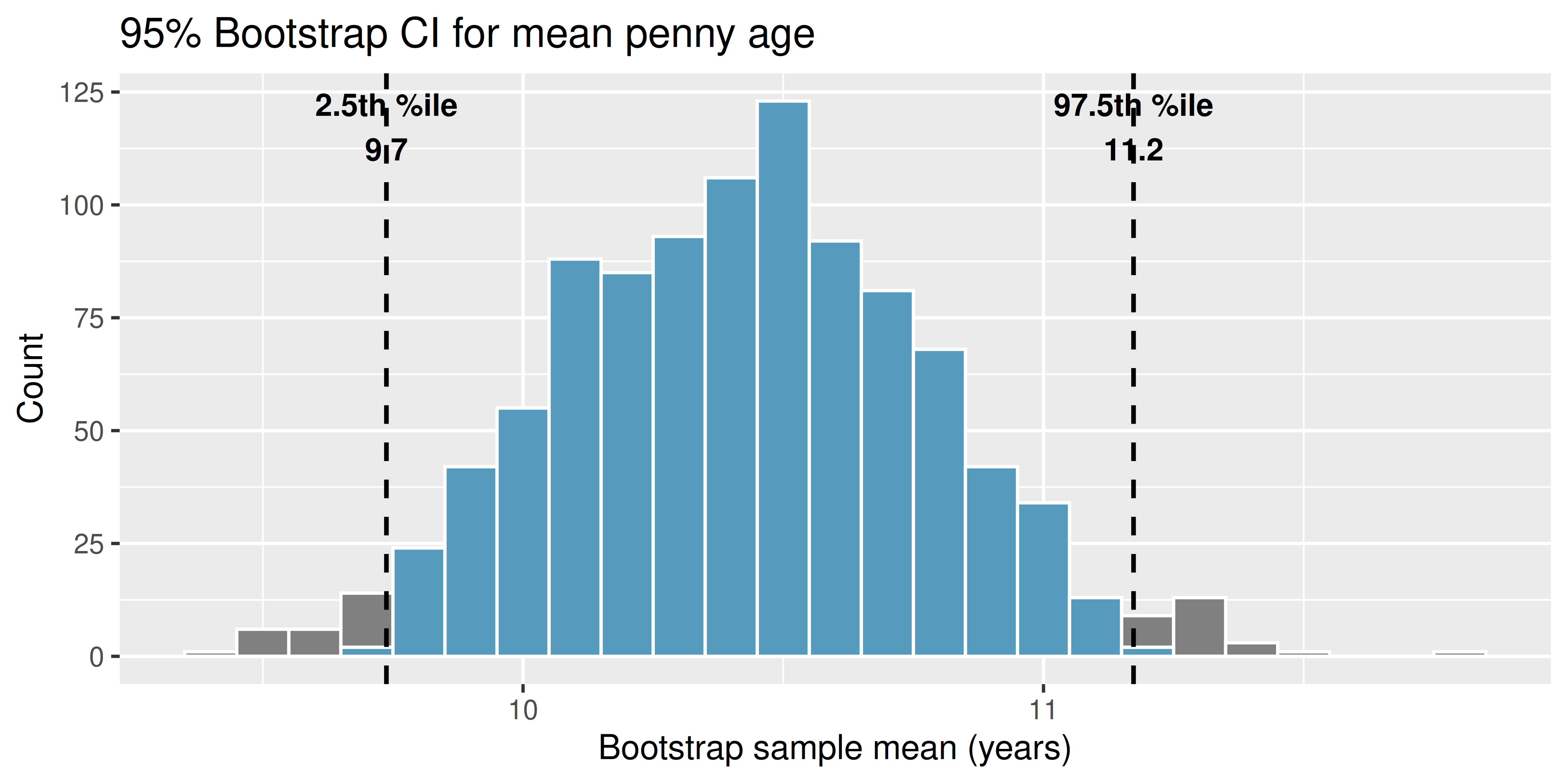
The 95% bootstrap confidence interval for the mean penny age is approximately (9.7, 11.2) years.

9.3 Interpreting a confidence interval

A confidence interval is a range of plausible values for the population parameter. A 95% confidence interval is constructed using a procedure that, when applied repeatedly to many different samples, captures the true parameter in approximately 95% of all intervals produced.

What “95% confident” means: If we repeated the entire study many times — collecting a new sample each time and computing a new 95% confidence interval — approximately 95% of those intervals would contain the true population parameter. Any single interval either contains the parameter or it doesn’t; the 95% refers to the long-run success rate of the procedure.

To illustrate the coverage concept, imagine we could treat our 648 pennies as if they were the entire population (with true mean \(\mu \approx 10.4\) years). We then draw 25 smaller random samples of 50 pennies each and build a bootstrap CI from each one. This lets us check whether each interval captures the “true” mean — something we can never do with real data, because we don’t know the true parameter.

Figure 9.4: Twenty-five 95% confidence intervals from 25 different random samples of pennies. The true population mean is shown as a vertical dashed line. Approximately 95% of intervals capture the true mean; a few (shown in red) miss it. Open in StatLens

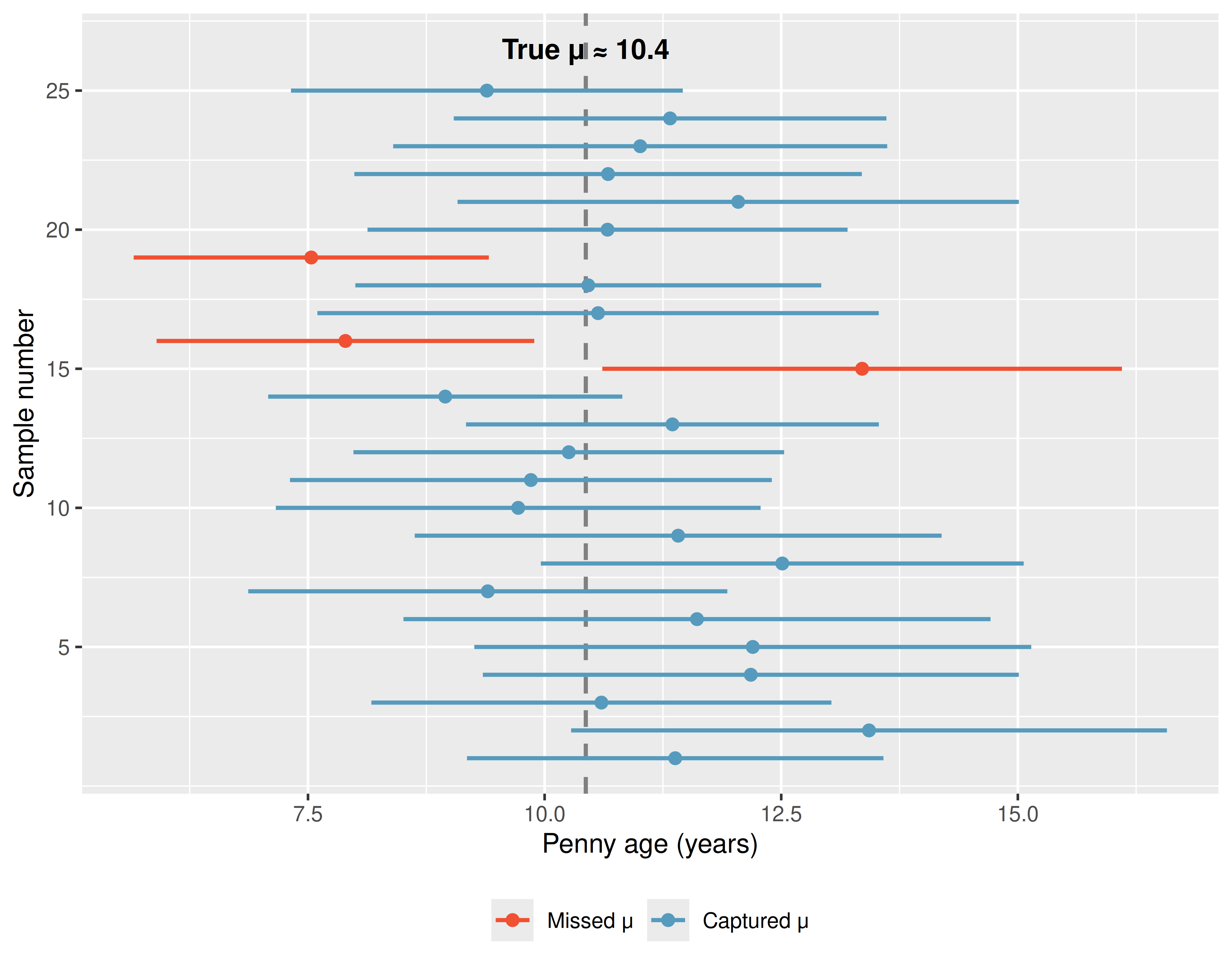
Each horizontal line in Figure 9.4 represents a 95% CI from a different sample. Most intervals (blue) capture the true mean, but a few (red) miss it entirely. Over many samples, roughly 95% of the intervals succeed. This is the meaning of “95% confidence.”

See it in action. Open the CI Coverage demo and keep drawing 95% confidence intervals from fresh samples of 50 pennies. Watch how most intervals (blue) capture the true mean while a few (red) miss — and how the running coverage rate settles near 95% as you accumulate more intervals. The moving image is the “95% confidence” concept in a way a static figure cannot be.

Common misinterpretation: “There is a 95% probability that the true mean is in this interval.” This statement treats the population mean as random and the interval as fixed. In fact, the population mean is fixed (we just don’t know it) and the interval is random (it depends on which sample we happened to collect).

A 95% bootstrap CI for the mean age of pennies in circulation is (9.7, 11.1). Which of the following interpretations is correct?

1. 95% of all pennies in circulation have ages between 9.7 and 11.1 years.
2. There is a 95% probability that the true mean penny age is between 9.7 and 11.1.
3. We are 95% confident that the true mean age of all pennies in circulation is between 9.7 and 11.1 years.

Show answer

Only (c) is correct. Statement (a) describes individual penny ages, not the mean. Statement (b) assigns a probability to the fixed parameter, which is incorrect. Statement (c) correctly describes confidence in the procedure.

9.4 The percentile method

The approach we’ve used is called the percentile method for bootstrap confidence intervals.

For a \((1 - \alpha) \times 100\%\) confidence interval using the percentile method:

• Lower bound = the \((\alpha/2) \times 100\)th percentile of the bootstrap distribution
• Upper bound = the \((1 - \alpha/2) \times 100\)th percentile of the bootstrap distribution

For a 95% CI (\(\alpha = 0.05\)): use the 2.5th and 97.5th percentiles. For a 90% CI (\(\alpha = 0.10\)): use the 5th and 95th percentiles. For a 99% CI (\(\alpha = 0.01\)): use the 0.5th and 99.5th percentiles.

If you increase the confidence level from 95% to 99%, what happens to the width of the confidence interval? Why?

Show answer

The interval gets wider. A 99% CI must capture the true parameter more often than a 95% CI, so it must cast a wider net. The 0.5th percentile is farther from the center than the 2.5th percentile.

9.5 The standard error method

The percentile method reads the confidence interval directly off the two tails of the bootstrap distribution. A second approach — the standard error method — instead summarizes the bootstrap distribution by its spread. It is the bridge to the formula-based confidence intervals we develop with the normal and \(t\) distributions in Unit 3.

The bootstrap standard error (SE) is the standard deviation of the bootstrap distribution. When the bootstrap distribution is roughly symmetric and bell-shaped, an approximate 95% confidence interval is

\[\text{point estimate} \pm 2 \times SE.\]

The multiplier 2 comes from the normal model: about 95% of a bell-shaped distribution falls within two standard deviations of its center. (The more precise multiplier is 1.96, which we begin using in Unit 3.)

For the penny ages, the observed sample mean is 10.4 years and the bootstrap standard error — the standard deviation of the 1,000 bootstrap means — is 0.36 years. The standard error 95% confidence interval is

\[10.4 \pm 2(0.36) = (9.7, \ 11.2) \text{ years}.\]

This is essentially the same interval we found with the percentile method — as we should expect, because the bootstrap distribution of the mean penny age is nearly symmetric.

Two methods, usually one answer. For a symmetric, bell-shaped bootstrap distribution, the percentile method and the standard error method give almost identical intervals. They can disagree when the bootstrap distribution is skewed — there the percentile method, which follows the actual shape of the distribution, is the safer choice. The standard error method matters because it connects directly to the formula-based confidence intervals of Unit 3, where the standard error comes from a formula instead of from resampling.

9.6 Medical consultant case study

People providing an organ for donation sometimes seek the help of a special medical consultant. These consultants assist the patient in all aspects of the surgery, with the goal of reducing the possibility of complications during the medical procedure and recovery.

One consultant tried to attract patients by noting the average complication rate for liver donor surgeries in the US is about 10%, but her clients have had only 3 complications in the 62 liver donor surgeries she has facilitated. She claims this is strong evidence that her work reduces complications.

We estimate the true complication rate \(p\) using the sample proportion: \(\hat{p} = 3/62 = 0.048\) (4.8%).

Is it possible to assess the consultant’s claim — that the reduction in complications is due to her work — using these data?

No. The claim is causal, but the data are observational. Patients who can afford a medical consultant may also afford better medical care overall, which could lead to a lower complication rate. We cannot establish causation here. But we can estimate the consultant’s true complication rate using a confidence interval.

To build a bootstrap CI for a proportion, we treat the 62 patients as marbles in a bag: 3 orange (complication) and 59 blue (no complication). We draw 62 marbles with replacement, compute \(\hat{p}^*_{boot}\), and repeat 10,000 times.

Figure 9.5: Bootstrap distribution of 10,000 resampled complication rates. The 95% CI extends from the 2.5th percentile to the 97.5th percentile. Because the interval includes 10%, we cannot conclude the consultant’s rate is lower than the national average. Open in StatLens

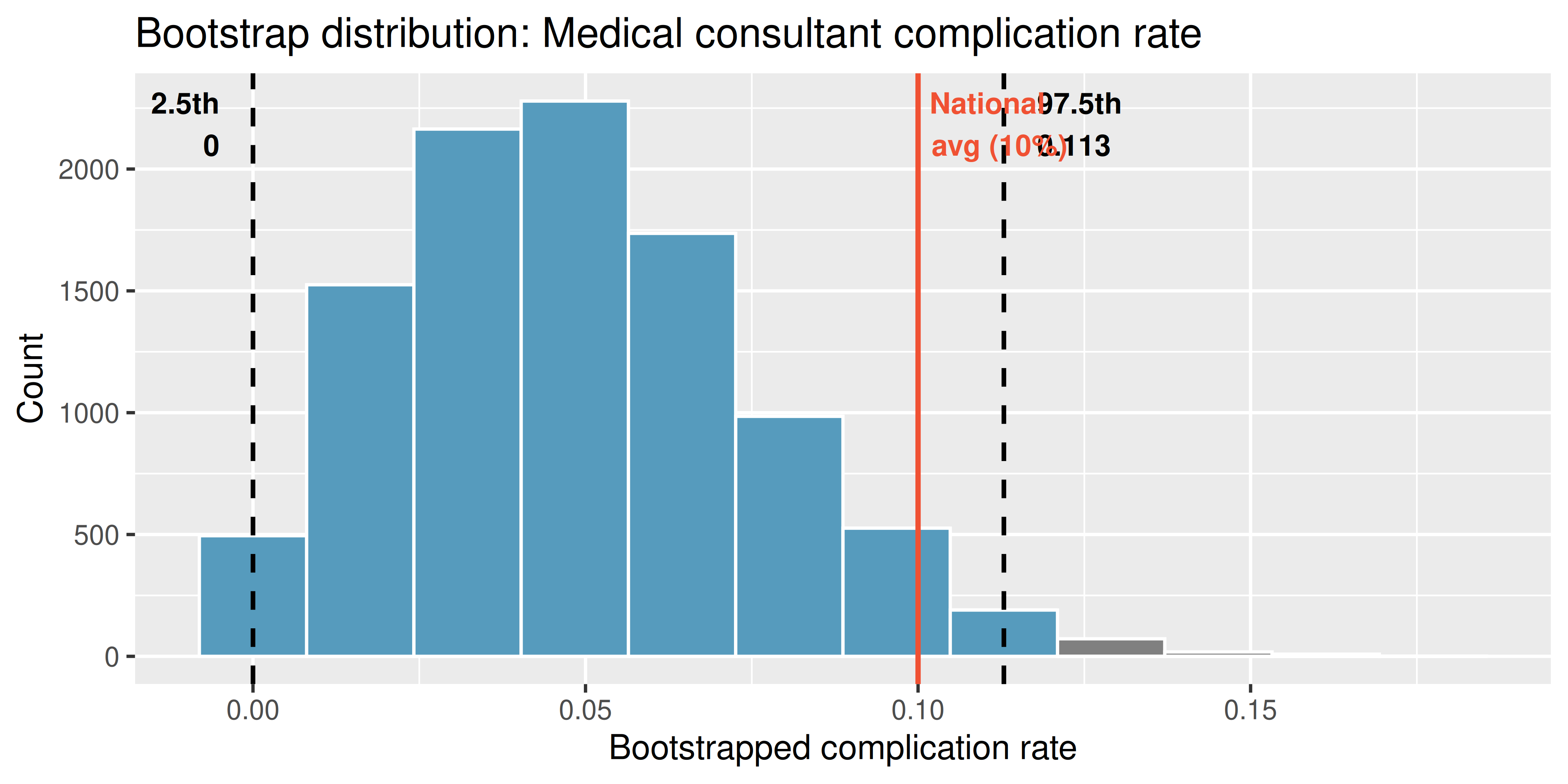
The 95% bootstrap CI is approximately (0, 0.113). The national average of 10% is right near the upper boundary of this interval — a borderline case. We certainly don’t have strong evidence that the consultant’s rate is lower than the national average. The sample is small (\(n = 62\)) and the CI is wide, so complication rates anywhere from 0% up to around 10% are plausible.

Because there are only 62 patients and each is either “complication” or “no complication,” the bootstrap proportions can only take values that are multiples of \(1/62\) (0, 1/62, 2/62, …). This discreteness means the CI boundary can only land on one of these values — it can’t fall smoothly between them. You may notice the CI upper bound jump between 6/62 \(\approx\) 0.097 and 7/62 \(\approx\) 0.113 depending on how many resamples you generate. This is normal with small-sample proportion data and is one reason why borderline conclusions should be stated cautiously. It also means the interval’s actual confidence level may differ from the nominal 95% — here, the true coverage is closer to 99% because the discrete boundaries force the interval to be wider than intended.

Predict → Do → Explain. Open the Medical Consultant Activity — the gated activity opens with a Predict step (commit to whether the 95% CI will include 10%, how discreteness will bite, and what changes when \(n\) triples), walks you through bootstrapping the consultant’s data at \(n = 62\) and then at larger \(n\) with the discreteness made visible at each stage, and closes with an Explain step where you articulate what “the CI includes 10%” does and does not let us conclude. Your predictions and explanation save locally in the tool, so you can leave the activity and return to your work on the same device.

Suppose the consultant had facilitated 620 surgeries (instead of 62) with the same complication rate of 4.8% (about 30 complications). How would the bootstrap CI change? Would the conclusion change?

Show answer

With 10 times as much data, the bootstrap distribution would be much narrower. The 95% CI would likely fall entirely below 10%, providing strong evidence that the consultant’s rate is lower. Larger samples give more precise estimates.

9.7 Tappers and listeners case study

A Stanford University graduate student named Elizabeth Newton conducted an experiment using a simple game: one person (the “tapper”) taps out a well-known song on a desk, and another person (the “listener”) tries to guess the song. About 50% of tappers expected the listener would guess correctly.

In Newton’s study, only 3 out of 120 listeners (\(\hat{p} = 3/120 = 0.025\)) guessed the tune correctly. What is the true proportion of listeners who can guess the song?

Figure 9.6: Bootstrap distribution for the proportion of listeners who guessed correctly. The 95% CI is far below the tappers’ expected success rate of 50%, providing very convincing evidence against the tappers’ expectation.

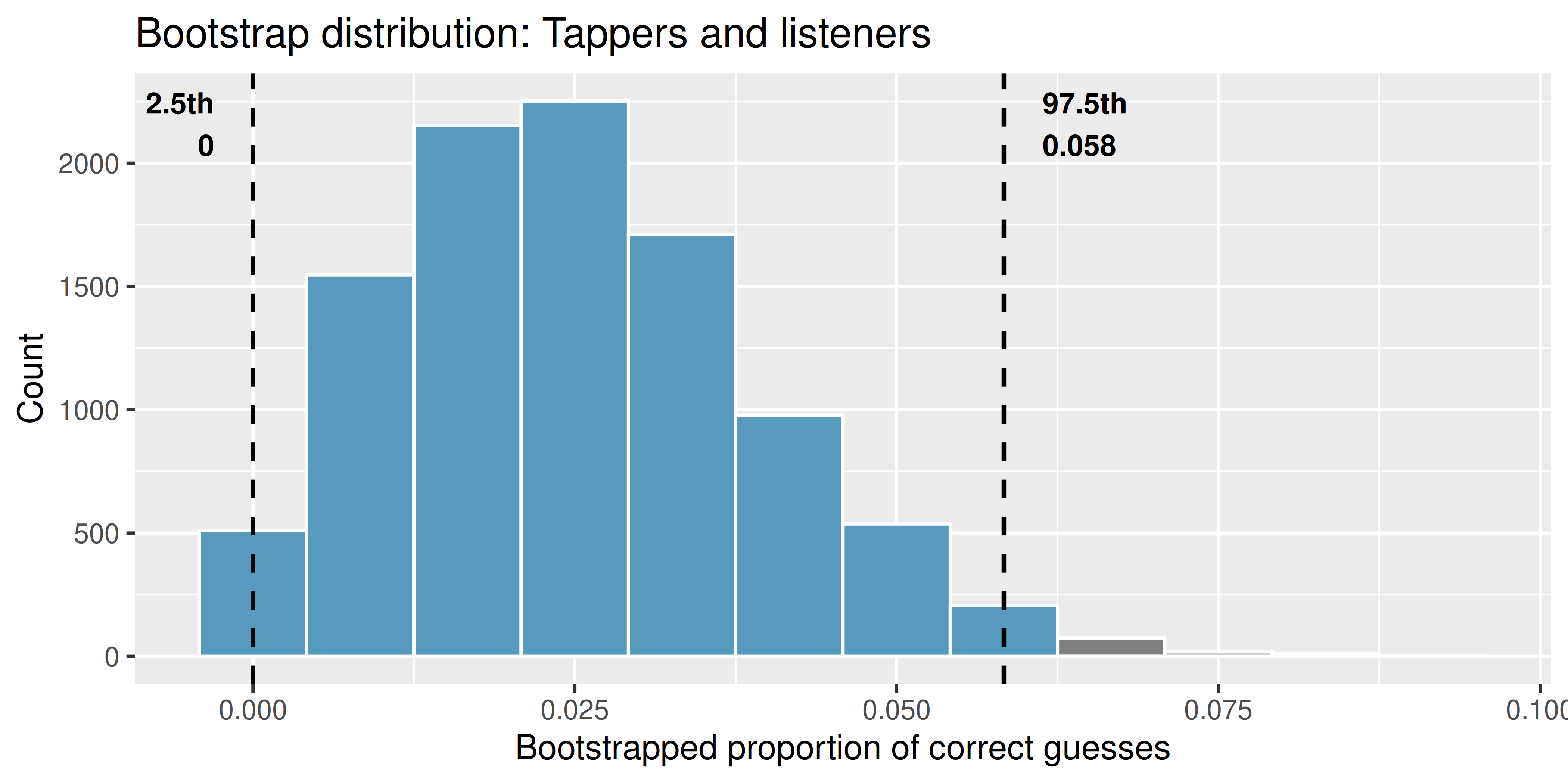
The 95% bootstrap CI is approximately (0, 0.058). The tappers’ expectation of 50% is nowhere near this interval — it provides very convincing evidence that listeners are far worse at guessing than tappers expect. This is an example of the “curse of knowledge”: once you know something, it’s hard to imagine not knowing it.

Do the data provide convincing evidence against the claim that 50% of listeners can guess the tapper’s tune?

Show answer

Yes, very convincing evidence. The value 50% (0.50) is far outside the 95% CI, and even far from the largest bootstrapped proportion. The data strongly suggest that the true success rate is much lower than 50%.

9.8 What affects the width of a CI?

Three factors control how wide a confidence interval is:

1. Sample size (\(n\)): Larger samples → narrower intervals (more information about the population)
2. Variability in the data: More spread → wider intervals (less precision)
3. Confidence level: Higher confidence → wider intervals (more certainty requires a wider net)

Figure 9.7: The effect of sample size on the bootstrap distribution. Larger samples produce narrower bootstrap distributions, leading to narrower confidence intervals. All three panels use the same population of penny ages. Open in StatLens

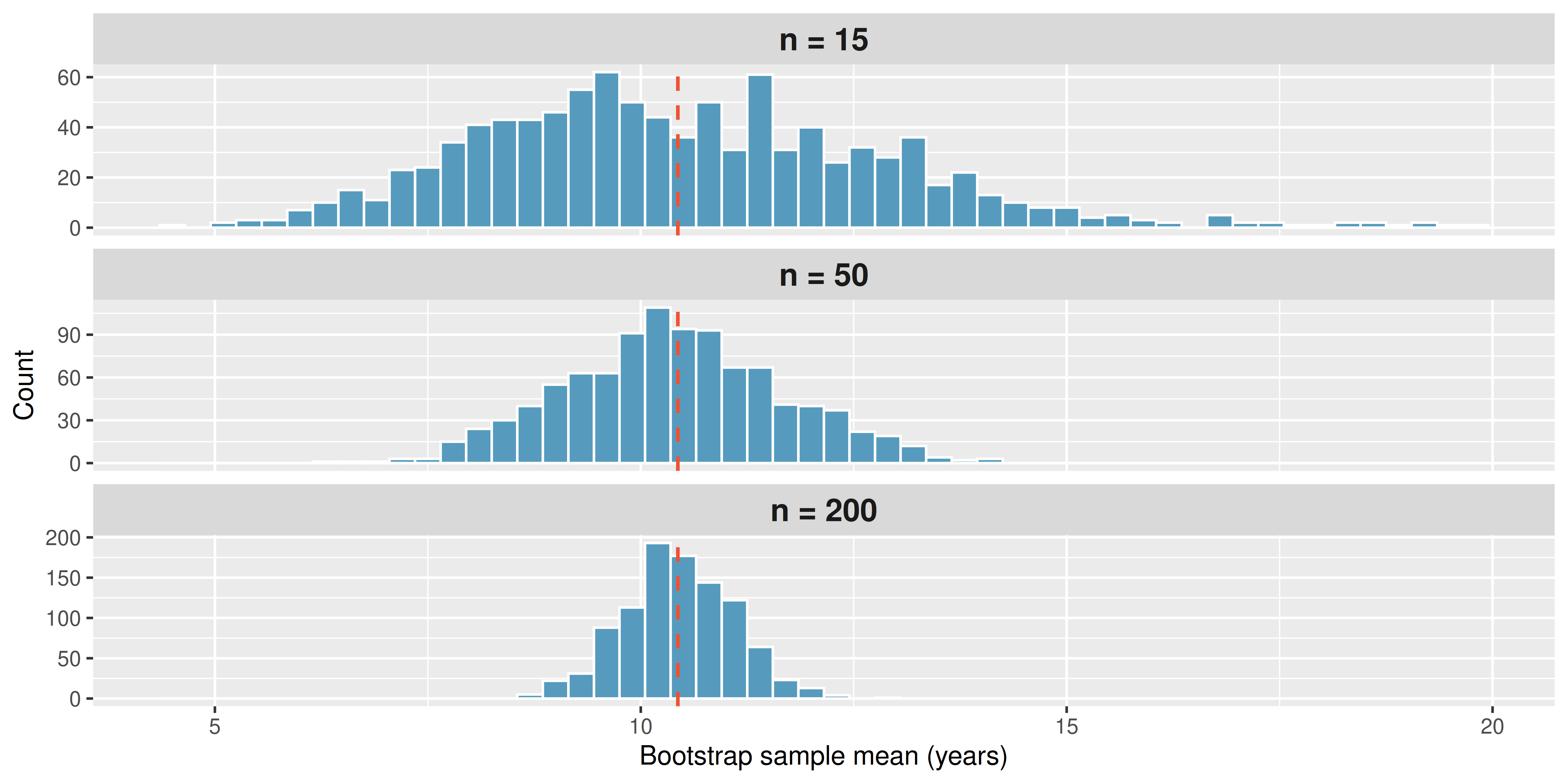
As sample size increases, the bootstrap distribution becomes tighter around the sample mean. This is why large studies produce more precise estimates than small ones.

Predict → Do → Explain. Open the Confidence Level Activity — the gated activity opens with a Predict step (commit to the direction, magnitude, and trade-off as you move the confidence level from 90% to 95% to 99%), walks you through those three intervals on the same bootstrap distribution with each frozen for direct width comparison, and closes with an Explain step where you articulate what “95% confident” means and why a wider net earns higher confidence. Your predictions and explanation save locally in the tool, so you can leave the activity and return to your work on the same device.

9.9 When does bootstrapping work?

Bootstrapping is remarkably flexible, but it does require some conditions to produce reliable intervals:

1. Independence: The observations in the sample should be independent of one another. This is usually satisfied when data come from a random sample or a randomized experiment.

2. Representative sample: The sample should be reasonably representative of the population. If the sample is biased (e.g., only volunteers), the bootstrap CI will reflect that bias.

3. Sufficient sample size: Very small samples (e.g., \(n < 10\)) may not contain enough information about the population’s shape. With small \(n\), the bootstrap distribution can be unreliable.

Bootstrapping does not require the population to follow a bell-shaped (normal) distribution. This is one of its greatest strengths compared to traditional formula-based methods, which often do require normality. The penny ages data are clearly right-skewed (Figure 9.1), yet the bootstrap procedure works perfectly well. The bootstrap lets the data “speak for themselves.”

A researcher surveys 8 of her friends about their study hours and computes a bootstrap CI. What condition is most clearly violated?

Show answer

Two conditions are violated: (1) the sample is a convenience sample of friends, not a random sample, so it may not be representative of the population, and (2) \(n = 8\) is quite small, making the bootstrap distribution potentially unreliable.

When neither bootstrap CI is enough. The two methods this chapter teaches — the percentile interval and the standard-error interval (statistic \(\pm z^{*} \cdot SE_{\text{boot}}\)) — are both starter tools, and they can go wrong in different ways. Be skeptical of either interval when:

• Sample size is small (below about 15–20). The bootstrap distribution can be lumpy and miss the shape of the true sampling distribution.
• The parameter sits near a boundary — a proportion near 0 or 1, a variance, an extreme quantile.
• The statistic is unusual — ratios, correlations, mins/maxes.

The two methods also have method-specific failure modes:

• The standard-error method assumes the bootstrap distribution is roughly symmetric and bell-shaped. When it isn’t, the formula forces symmetry the data don’t have and can push endpoints outside the parameter space (a negative bound for a proportion, for example).
• The percentile method respects skew but can under-cover the parameter on the “long-tail” side of a strongly skewed bootstrap distribution.

When any of these apply, professional practice reaches past both methods — most commonly to the BCa (bias-corrected and accelerated) interval, which corrects for both bias and skew in the bootstrap distribution. BCa is available in StatLens under expert mode and in R via boot::boot.ci(..., type = "bca"). Hesterberg’s “What Teachers Should Know About the Bootstrap” (The American Statistician, 2015) is the readable reference for when each method applies.

For this course we stay with these two methods — they are the simplest defensible tools that keep the simulation logic in view. Recognize their limits: they are starters, not the final word.

9.10 Bootstrap CI for other statistics

The beauty of bootstrapping is its generality. The same resampling logic works for any statistic, not just the mean:

• Median: Resample → compute median → repeat → percentile CI
• Proportion: Resample → compute proportion → repeat → percentile CI
• Standard deviation: Resample → compute SD → repeat → percentile CI
• Difference in means: Resample from each group → compute difference → repeat → percentile CI

This is a powerful advantage. Many statistics (like the median or the difference in medians) don’t have convenient formulas for their standard error. Bootstrapping handles them all the same way.

See it in action. Open the Bootstrap CI tool with penny ages and switch the statistic dropdown between the mean, median, standard deviation, Q1, and Q3. Same data, same resampling procedure — different summaries. Notice which statistics produce narrow, symmetric bootstrap distributions and which produce wide or skewed ones.

9.11 Chapter review

9.11.1 Summary

• The bootstrap constructs a confidence interval by resampling with replacement from the original sample.
• The bootstrap distribution approximates the sampling distribution of the statistic.
• The percentile method uses the middle \((1 - \alpha) \times 100\%\) of the bootstrap distribution as the CI.
• The standard error method uses point estimate \(\pm\, 2 \times SE\), where the SE is the standard deviation of the bootstrap distribution; it agrees with the percentile method for symmetric distributions and bridges to the formula-based intervals of Unit 3.
• A 95% confidence interval means that if we repeated the study many times, about 95% of the resulting intervals would capture the true parameter.
• CI width depends on sample size, data variability, and confidence level.
• Bootstrap CIs work for any statistic — means, medians, proportions, differences, and more.
• Bootstrapping requires independent observations from a representative sample with sufficient sample size, but does not require the population to be bell-shaped (normal).

9.11.2 Key terms

• Bootstrap resample
• Bootstrap statistic
• Bootstrap distribution
• Confidence interval
• Confidence level
• Percentile method
• Standard error method
• Bootstrap standard error
• Point estimate
• Parameter
• Sampling with replacement

9.12 Exercises

The StatLens Exercises (1–14) use interactive simulation tools — open the provided links and explore. The Practice Exercises (15–22) use static figures for additional practice. Answers to odd-numbered exercises are provided in the Exercise Solutions appendix at the back of the book.

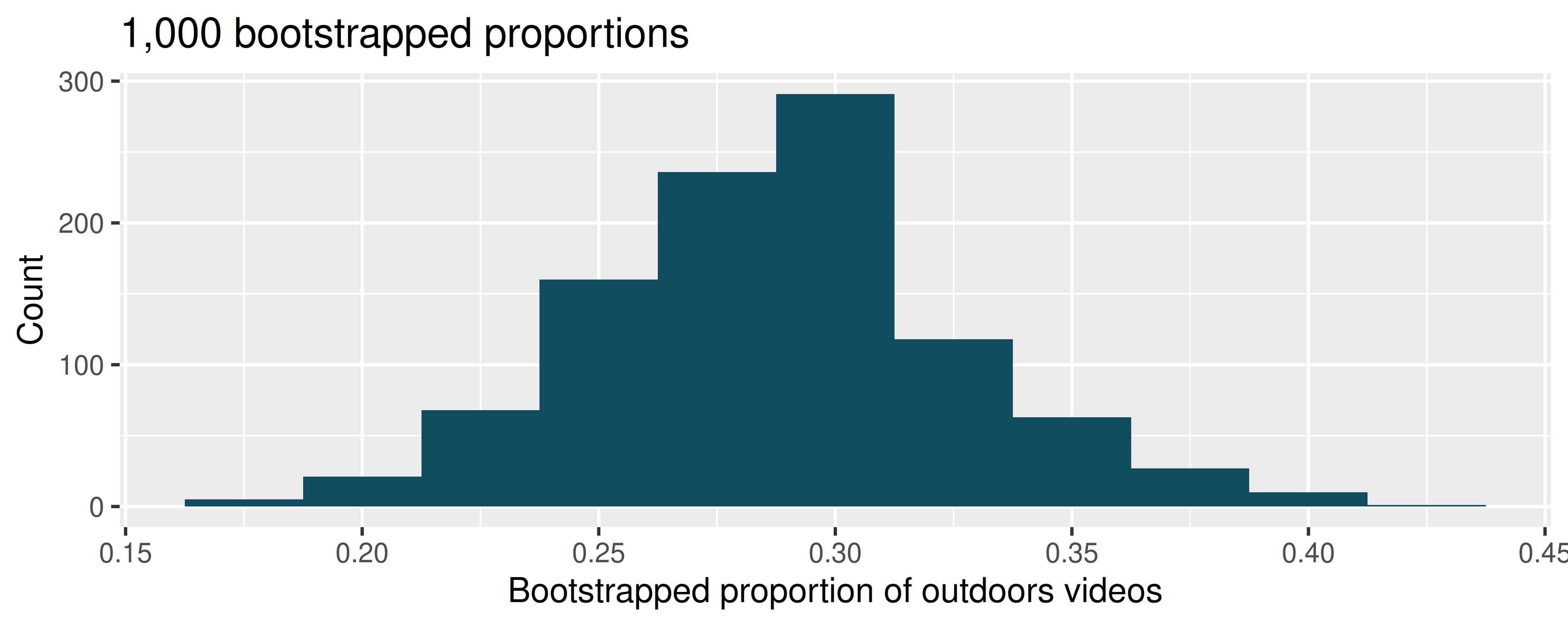
1. Outside YouTube videos. Let’s say that you want to estimate the proportion of YouTube videos which take place outside (define “outside” to be if any part of the video takes place outdoors). You take a random sample of 128 YouTube videos and determine that 37 of them take place outside. You’d like to estimate the proportion of all YouTube videos which take place outside, so you decide to create a bootstrap interval from the original sample of 128 videos.

1. Describe in words the relevant statistic and parameter for this problem. If you know the numerical value for either one, provide it. If you don’t know the numerical value, explain why the value is unknown.

2. What notation is used to describe, respectively, the statistic and the parameter?

3. If using software to bootstrap the original dataset, what is the statistic calculated on each bootstrap sample?

4. When creating a bootstrap sampling distribution (histogram) of the bootstrapped sample proportions, where should the center of the histogram lie?

5. The histogram provides a bootstrap sampling distribution for the sample proportion (with 1000 bootstrap repetitions). Using the histogram, estimate a 90% confidence interval for the proportion of YouTube videos which take place outdoors.

6. Interpret the confidence interval in context of the data.

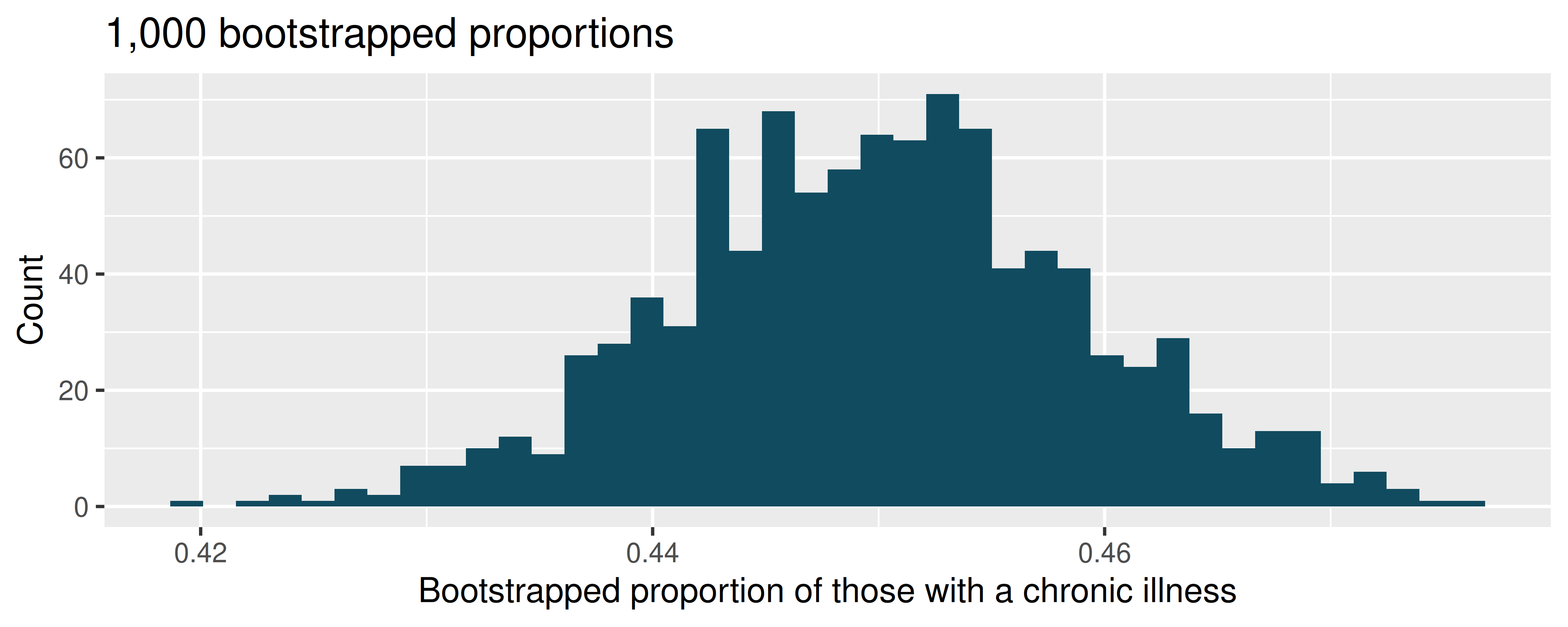
2. Chronic illness. In 2012 the Pew Research Foundation reported that “45% of US adults report that they live with one or more chronic conditions.” However, this value was based on a sample, so it may not be a perfect estimate for the population parameter of interest on its own. The study was based on a sample of 3014 adults. Below is a distribution of 1000 bootstrapped sample proportions from the Pew dataset. (Pew Research Center 2013) Using the distribution of 1,000 bootstrapped proportions, approximate a 92% confidence interval for the true proportion of US adults who live with one or more chronic conditions and interpret it.

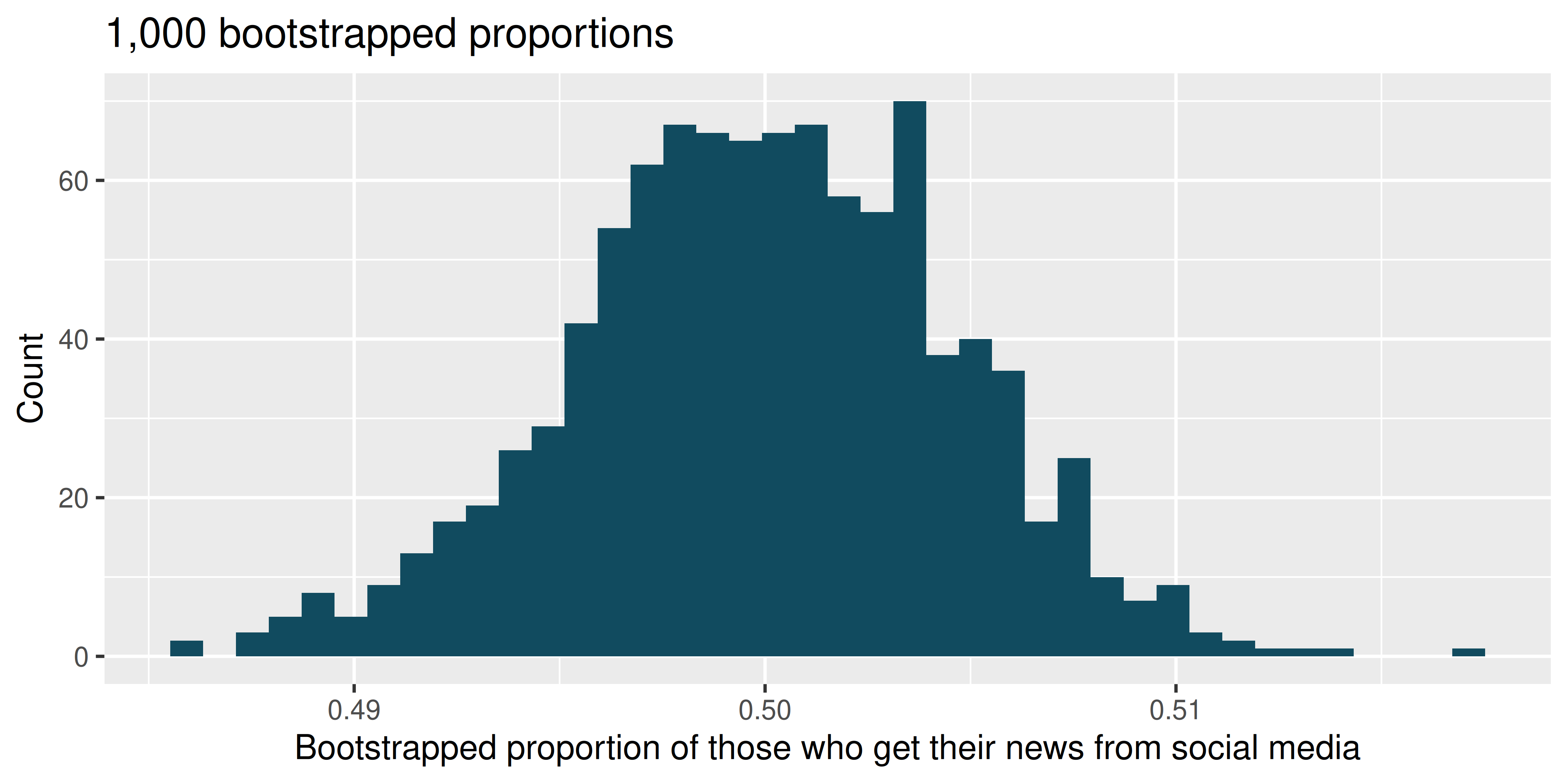
3. Social media users and news, bootstrapping. A poll conducted in 2022 found that 50% of U.S. adults get news from social media sometimes or often. However, the value was based on a sample, so it may not be a perfect estimate for the population parameter of interest on its own. The study was based on a sample of 12,147 adults. Below is a distribution of 1,000 bootstrapped sample proportions from the Pew dataset. (Pew Research Center 2022) Using the distribution of 1,000 bootstrapped proportions, approximate a 98% confidence interval for the true proportion of US adult social media users (in 2022) who get at least some of their news from Twitter. Interpret the interval in the context of the problem.

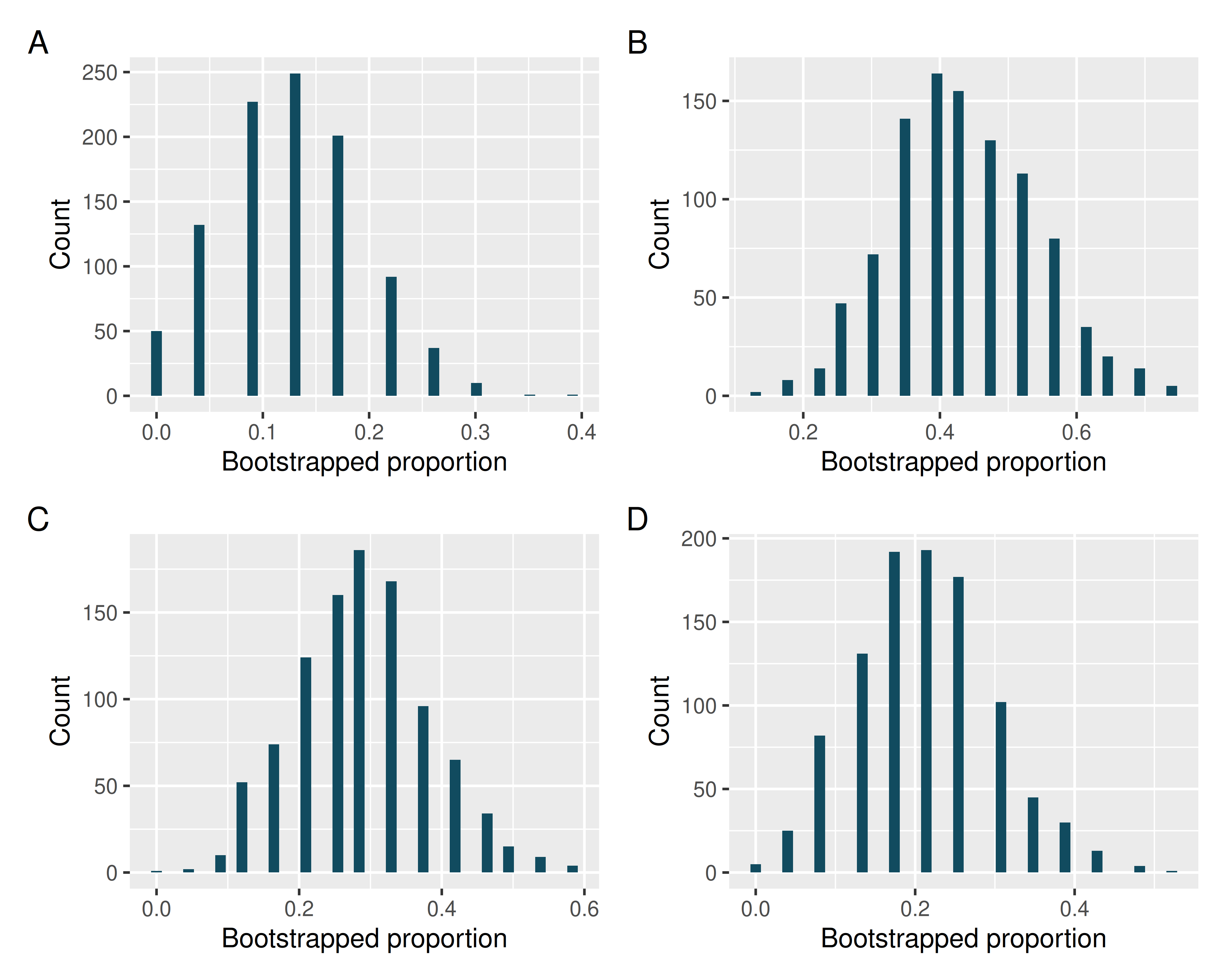
4. Bootstrap distributions of \(\hat{p}\), I. Each of the following four distributions was created using a different dataset. Each dataset was based on \(n=23\) observations. The original datasets had the following proportions of successes: \[\hat{p} = 0.13 \ \ \hat{p} = 0.22 \ \ \hat{p} = 0.30 \ \ \hat{p} = 0.43.\] Match each histogram with the original data proportion of success.

5. Bootstrap distributions of \(\hat{p}\), II. Each of the following four distributions was created using a different dataset. Each dataset was based on \(n=23\) observations.

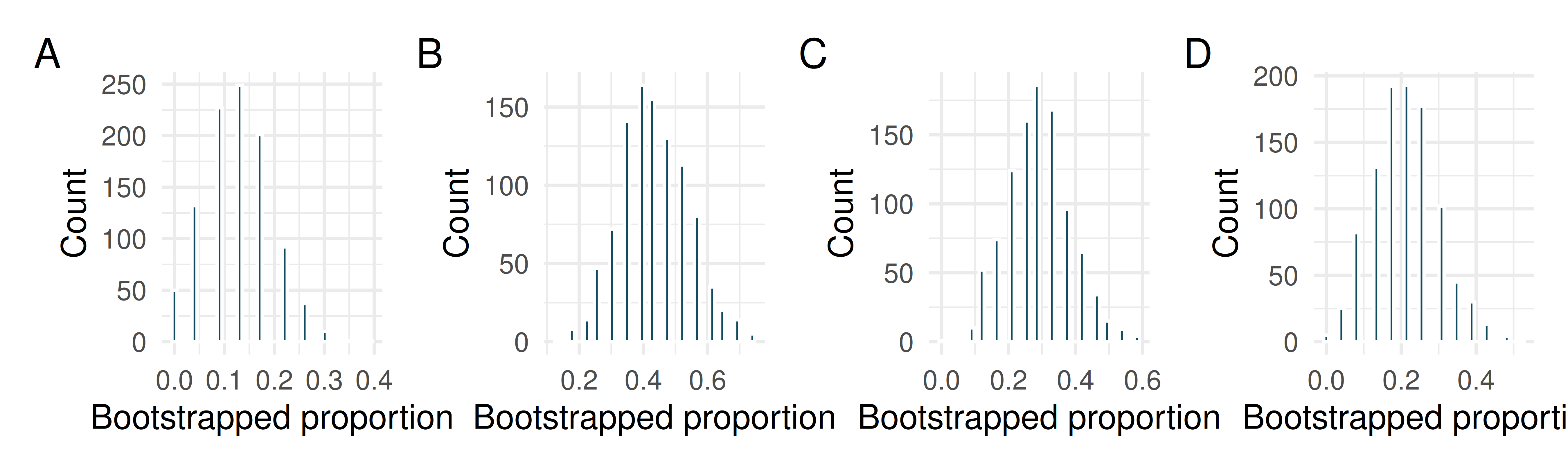
Consider each of the following values for the true popluation \(p\) (proportion of success). Datasets A, B, C, D were bootstrapped 1000 times, with bootstrap proportions as given in the histograms provided. For each parameter value, list the datasets which could plausibly have come from that population. (Hint: there may be more than one dataset for each parameter value.)

1. \(p = 0.05\)

2. \(p = 0.25\)

3. \(p = 0.45\)

4. \(p = 0.55\)

5. \(p = 0.75\)

6. Bootstrap distributions of \(\hat{p}\), III. Each of the following four distributions was created using a different dataset. Each dataset had the same proportion of successes \((\hat{p} = 0.4)\) but a different sample size. The four datasets were given by \(n = 10, 100, 500\), and \(1000\).

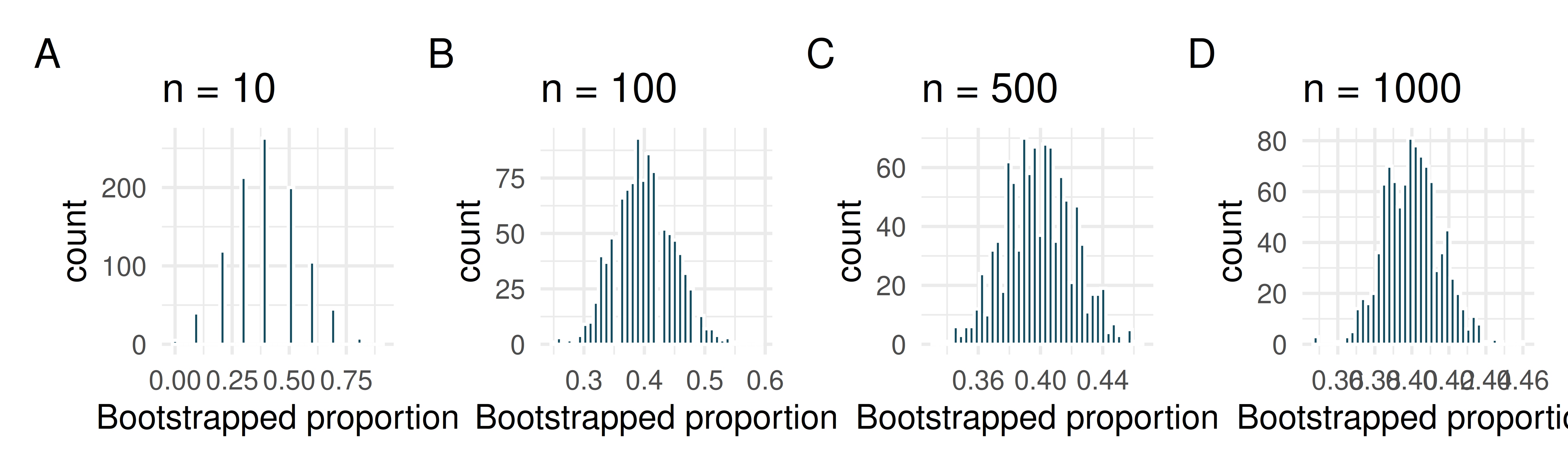
Consider each of the following values for the true popluation \(p\) (proportion of success). Datasets A, B, C, D were bootstrapped 1000 times, with bootstrap proportions as given in the histograms provided. For each parameter value, list the datasets which could plausibly have come from that population. (Hint: there may be more than one dataset for each parameter value.)

1. \(p = 0.05\)

2. \(p = 0.25\)

3. \(p = 0.45\)

4. \(p = 0.55\)

5. \(p = 0.75\)

7. Cyberbullying rates. Teens were surveyed about cyberbullying, and 54% to 64% reported experiencing cyberbullying (95% confidence interval). Answer the following questions based on this interval. (Pew Research Center 2018)

1. A newspaper claims that a majority of teens have experienced cyberbullying. Is this claim supported by the confidence interval? Explain your reasoning.

2. A researcher conjectured that 70% of teens have experienced cyberbullying. Is this claim supported by the confidence interval? Explain your reasoning.

3. Without actually calculating the interval, determine if the claim of the researcher from part (b) would be supported based on a 90% confidence interval?

8. Waiting at an ER. A 95% confidence interval for the mean waiting time at an emergency room (ER) of (128 minutes, 147 minutes). Answer the following questions based on this interval.

1. A local newspaper claims that the average waiting time at this ER exceeds 3 hours. Is this claim supported by the confidence interval? Explain your reasoning.

2. The Dean of Medicine at this hospital claims the average wait time is 2.2 hours. Is this claim supported by the confidence interval? Explain your reasoning.

3. Without actually calculating the interval, determine if the claim of the Dean from part (b) would be supported based on a 99% confidence interval?

9. Percentile or standard-error method? For each of the following bootstrap distributions, decide whether the percentile method and the standard-error method would give roughly the same 95% CI, or whether one is more trustworthy. Explain in one sentence.

1. The bootstrap distribution of the sample mean is roughly symmetric and bell-shaped, centered near the observed statistic.

2. The bootstrap distribution of the sample median is strongly right-skewed with a long upper tail.

3. The bootstrap distribution of a sample proportion \(\hat{p}\) is bounded (values can’t exceed 1) and pushed up against the upper boundary near \(\hat{p} = 0.95\).

4. A study has \(n = 12\); the bootstrap distribution looks lumpy and irregular but is roughly centered.

5. In one sentence, explain the underlying reason the two methods can disagree.

StatLens Exercises

These exercises focus on the parts of bootstrap inference a calculator can’t do for you: framing the question, picking the right resampling scheme, reading the bootstrap distribution, and interpreting a confidence interval without falling into the standard traps. Let StatLens do the arithmetic.

1. Frame the question. A coffee shop wants to estimate the median wait time at its drive-through. The owner records a random sample of \(n = 80\) wait times in seconds.

   1. What is the parameter of interest? Describe it in words and give a symbol.
   2. Why is a bootstrap confidence interval especially well-suited to the median compared to the mean?
   3. Should the resulting bootstrap CI be percentile-based or standard-error-based, and how would you choose between them?

2. Choose the resampling scheme. For each scenario, name the resampling — resample with replacement from one sample (one mean/median/SD/proportion), resample within each group (two means/proportions, independent groups), resample paired-difference values (paired data), or the bootstrap doesn’t apply here (and why).

   1. Estimate the mean weight of a single bag of coffee from 30 weighed bags.
   2. Estimate the difference in mean delivery time between two couriers based on 25 deliveries each.
   3. Estimate the difference in the proportion of customers who return for a second visit after two different welcome promotions (random assignment).
   4. Estimate the standard deviation of completion times in a single sample of 60 jobs.
   5. Estimate the maximum age in a population from a random sample of 50 people.

3. Read the bootstrap distribution. Open the Bootstrap CI for One Proportion with the medical consultant data (62 patients, 3 complications, \(\hat{p} \approx 0.048\)). Generate 10000 resamples.

   1. Describe the shape, center, and spread of the bootstrap distribution. What feature of the data (small \(\hat{p}\)) is responsible for the shape?
   2. Read off the 95% percentile interval. Does it contain the national average of 0.10?
   3. If you instead built a symmetric 95% interval as \(\hat{p} \pm 2 \cdot \text{SE}_{\text{boot}}\), what would go wrong? Sketch what that interval would look like next to the percentile interval.

4. Run it and interpret it. Open any one-variable numeric dataset in the Bootstrap CI for One Mean tool and generate 5000 resamples at 95% confidence.

   1. Report the 95% percentile interval StatLens gives you.

   2. Write a one-sentence conclusion in context, naming the population and the units.

   3. Which statement is the correct interpretation of the interval?

      1. There is a 95% probability that the true mean lies in this interval.
      2. If the study were repeated many times, about 95% of the intervals built this way would contain the true mean.
      3. 95% of the observations in our sample fall within this interval.
      4. 95% of the bootstrap resamples have means in this interval.

   4. Change the confidence level to 99% and re-run. Does the interval get wider or narrower? Why?

5. Simulation vs. analytic — where the bootstrap shines. The normal-approximation formula and the bootstrap are two routes to the same confidence interval. Sometimes they nearly coincide; sometimes they don’t.

   First a well-behaved case. Open a moderately large, roughly symmetric numeric dataset in both the Bootstrap CI for One Mean and the One-Sample \(t\) tool.

   1. Record the 95% interval from each. How close are they?

   Now the troublesome case. Pick a small, skewed dataset (you can paste in your own).

   2. Report the 95% intervals from each tool. Are they as close as in (a)? Where do they differ — in the midpoint, the width, or both?
   3. Explain the pattern. Why do the bootstrap percentile interval and the \(t\)-interval agree on well-behaved data but diverge on small skewed data? Tie your explanation to (i) the symmetry of the \(t\)-interval and (ii) the bootstrap’s ability to follow the shape of the sampling distribution.
   4. A student says: “The \(t\)-interval and the bootstrap interval disagree, so one of them must be wrong.” Why is that the wrong framing? Which interval should you trust more when they disagree, and why?

Pew Research Center. 2013. “The Diagnosis Difference.” https://www.openintro.org/go?id=textbook-pew-2013-diagnosis-difference.

———. 2018. “A Majority of Teens Have Experienced Some Form of Cyberbullying, Data Collected March 7 - April 10, 2018.” https://www.openintro.org/go?id=textbook-pew-2018-cyberbullying.

———. 2022. “News Consumption Across Digital Platforms.” https://www.pewresearch.org/journalism/fact-sheet/news-platform-fact-sheet/pj_2022-09-20_news-platforms_0-03b/.