Project: Association Between Two Categorical Variables (AI version)

Project — Chi-Square Test of Independence. Carry out the analysis in Jamovi (or R) and communicate the result. The graded skills are framing the association question, checking the expected-count condition, and interpreting the test in context.

The question

AI coding tools (ChatGPT, Copilot, and the like) swept into software work almost overnight. A natural question: is adoption uniform, or does it depend on who you are?

Among developers, is using AI tools associated with age?

The data

ai_tool_use.csv is a random sample of 600 developers from the Stack Overflow Annual Developer Survey (2024). You’ll use two categorical variables: ai_use (Yes, Not yet, but plan to, No — do you use AI tools in your development work?) and age_group (18-24, 25-34, 35-44, 45+).

Data source & license. Stack Overflow Annual Developer Survey 2024 (via the TidyTuesday project), used under the Open Database License (ODbL) 1.0. This excerpt is a derived subset; it is shared under ODbL — an exception to this book’s CC BY-SA license.

Plan it first

1. Variables. Confirm both variables are categorical and give the size of the table (rows × columns).
2. Hypotheses. State \(H_0\) and \(H_A\) for a test of independence in words (AI-tool use and age are independent vs. associated).
3. Eyeball it. Look at the row percentages (the AI-use mix within each age group). Can you tell for sure whether adoption depends on age, or could the differences be chance? This is the judgment the test makes rigorous.
4. Procedure & condition. Two categorical variables, “are they associated?” → chi-square test of independence. It needs expected counts that aren’t too small (a common rule: each ≥ 5) — what will you check?

Do the analysis

Jamovi

1. Open ai_tool_use.csv.
2. Frequencies → Independent Samples (χ² test of association). Rows: age_group; Columns: ai_use.
3. Request the χ² test, expected counts, and row percentages.
4. Read off the table, confirm expected counts are large enough, and record χ² and the p-value.

(Jamovi screenshots to be added.)

R

library(infer)
library(dplyr)
library(readr)
library(ggplot2)

ai <- read_csv("../datasets/ai_tool_use.csv")

# Order the categories
ai <- ai |>
  mutate(age_group = factor(age_group, levels = c("18-24", "25-34", "35-44", "45+")),
         ai_use     = factor(ai_use, levels = c("Yes", "Not yet, but plan to", "No")))

# Contingency table
tab <- table(ai$age_group, ai$ai_use)
tab

       
        Yes Not yet, but plan to  No
  18-24  96                   16  23
  25-34 136                   19  44
  35-44  94                   26  42
  45+    51                   24  29

# Row percentages: the AI-use mix within each age group (try to eyeball it)
round(100 * prop.table(tab, 1), 0)

       
        Yes Not yet, but plan to No
  18-24  71                   12 17
  25-34  68                   10 22
  35-44  58                   16 26
  45+    49                   23 28

# Chi-square test of independence (infer)
ai |> chisq_test(ai_use ~ age_group)

# A tibble: 1 × 3
  statistic chisq_df p_value
      <dbl>    <int>   <dbl>
1      19.8        6 0.00306

# Condition check: smallest expected count (rule of thumb: each >= 5)
cat("Smallest expected count:", round(min(chisq.test(tab)$expected), 1), "\n")

Smallest expected count: 14.7 

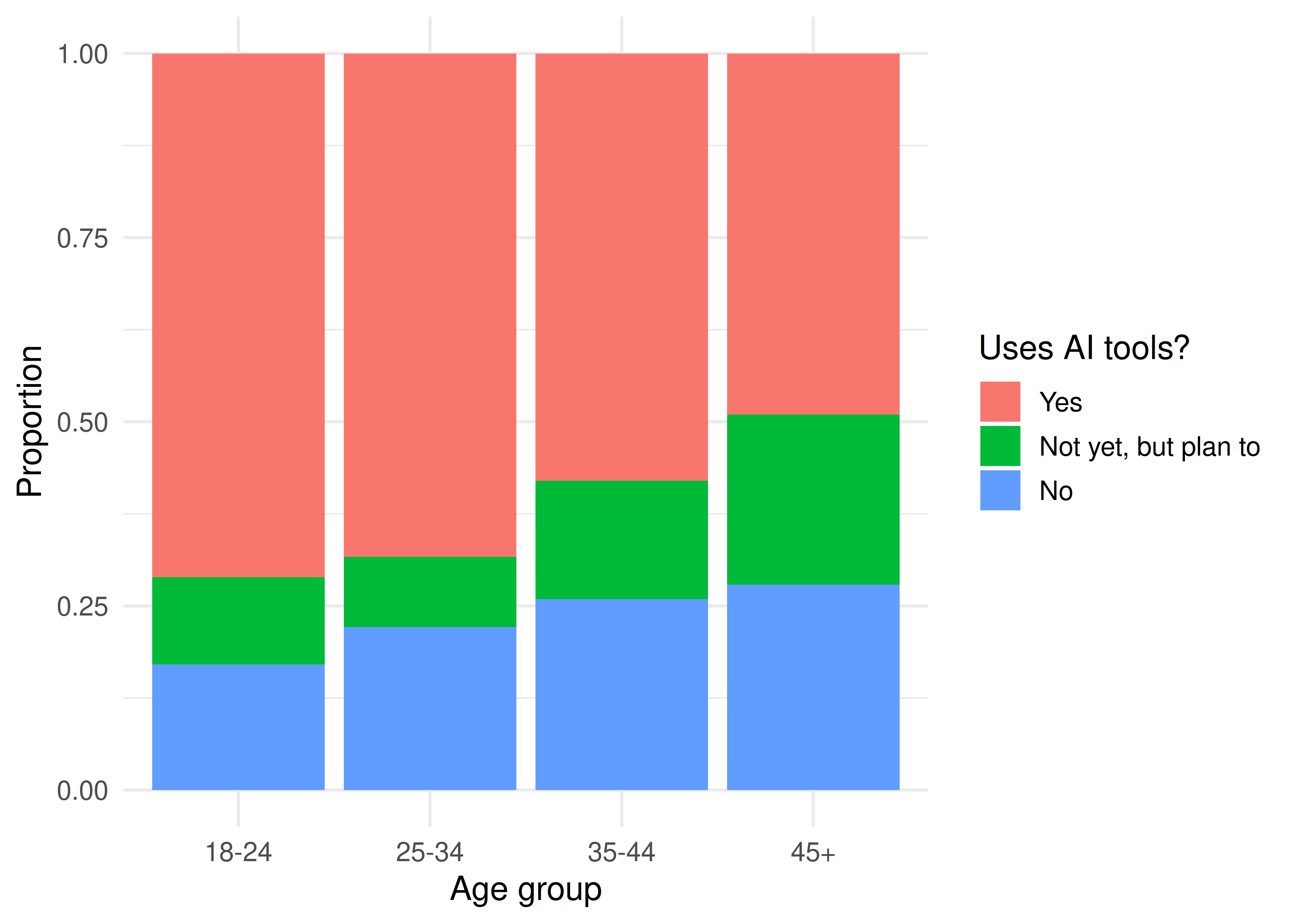
ggplot(ai, aes(age_group, fill = ai_use)) +
  geom_bar(position = "fill") +
  labs(x = "Age group", y = "Proportion", fill = "Uses AI tools?") +
  theme_minimal(base_size = 13)

AI-tool use by age group in a sample of 600 developers. Younger developers adopt AI tools more — but is the difference real or noise?

Your deliverable

Submit a short report containing all of:

1. Graphic — a labeled stacked (or side-by-side) bar chart showing the AI-use mix by age group.
2. Numerical result — the contingency table, the χ² statistic, the degrees of freedom, and the p-value.
3. Conditions — one sentence confirming the expected counts are large enough for the chi-square approximation.
4. Conclusion in context — 3–4 sentences: is there discernible evidence that AI-tool use is associated with age? Describe the pattern (who adopts most?), note how the test settled what the percentages alone left uncertain, and stress that association is not causation.
5. One limitation — e.g., this samples developers who chose to take one survey; results may not generalize to all workers, and attitudes change fast.

How it’s graded

Criterion	What we look for
Appropriate, labeled graphic	AI-use mix by group, axes/legend labeled
Procedure & conditions	chi-square independence identified; expected counts checked
Correct numerical result	table, χ², df, p-value reported correctly
Conclusion in context	discernibility + the age pattern + association ≠ causation
Communication	clear, correct interpretation

Warm up first. Explore expected counts and the χ² statistic in the Chi-Square tool before writing your report.