13 Confidence Intervals for Means
In the bootstrap confidence intervals chapter, we used bootstrapping to construct confidence intervals – a flexible, simulation-based approach that works well in many settings. In the normal approximation chapter, we saw that sampling distributions are often well approximated by the normal distribution. For means, however, we encounter a complication: the population standard deviation \(\sigma\) is almost never known, and estimating it with the sample standard deviation \(s\) introduces extra uncertainty. To account for this, we use a slightly different bell-shaped distribution called the \(t\)-distribution. In this chapter, we develop \(t\)-based confidence intervals for one mean, the difference between two independent means, and the mean of paired differences.
13.1 The \(t\)-distribution
13.1.1 Why not the normal distribution?
Earlier we used the normal distribution to model sampling distributions, and in the previous chapter we applied it to proportions, where the standard error formula \(SE = \sqrt{\hat{p}(1 - \hat{p})/n}\) depends only on the sample proportion and the sample size – both of which are known. For means, the standard error is \(SE = \sigma / \sqrt{n}\), which depends on \(\sigma\), the population standard deviation. Since we rarely know \(\sigma\), we estimate it using the sample standard deviation \(s\):
\[SE \approx \frac{s}{\sqrt{n}}\]
This substitution introduces additional uncertainty, especially in small samples. When \(n\) is small, \(s\) can be a poor estimate of \(\sigma\), and the normal model underestimates how variable the statistic really is. The \(t\)-distribution corrects for this.
13.1.2 Properties of the \(t\)-distribution
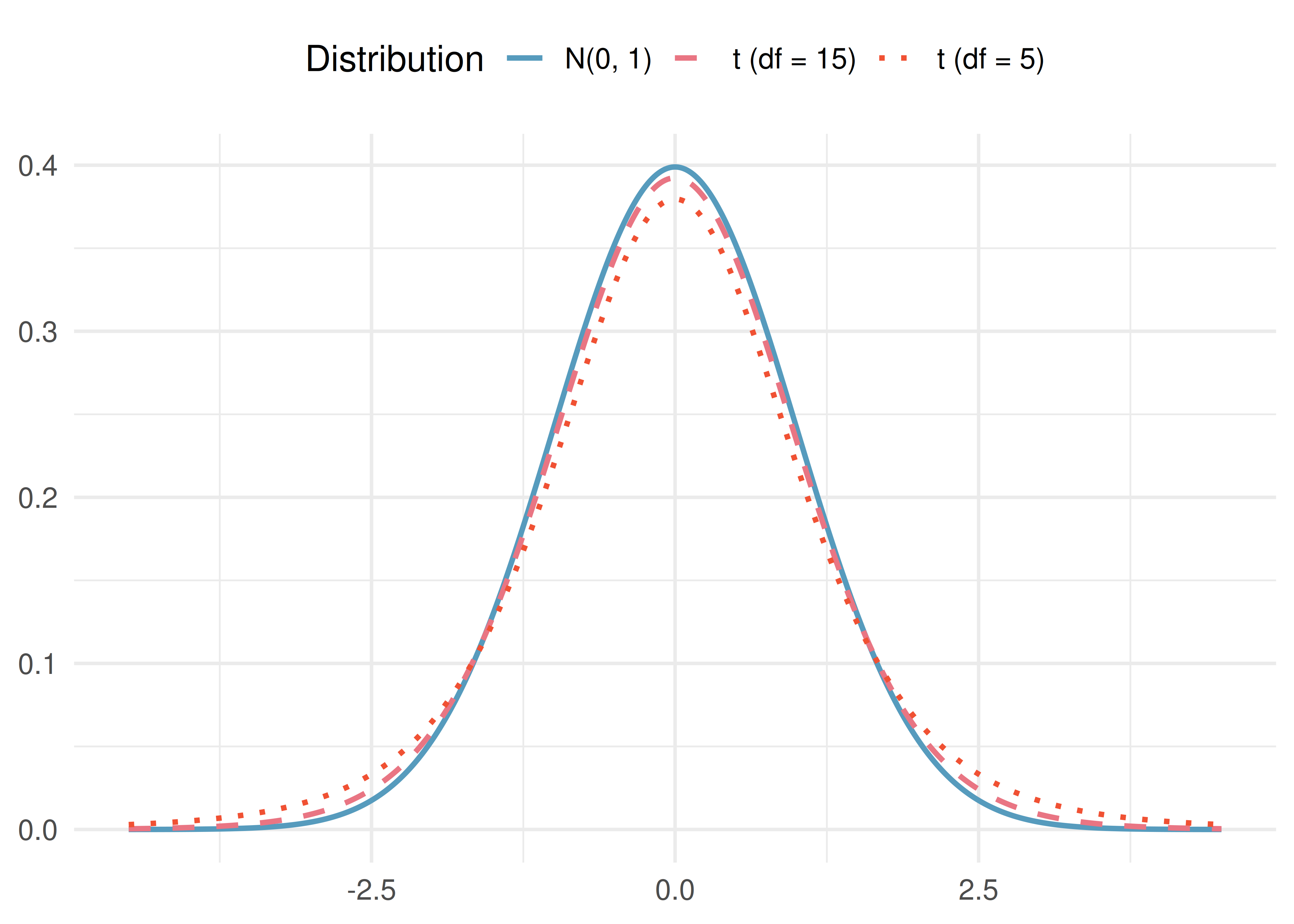
The \(t\)-distribution is a bell-shaped, symmetric distribution that is similar to the normal distribution but has heavier tails (more probability in the extremes). The exact shape of the \(t\)-distribution depends on a parameter called the degrees of freedom (df).
- When \(df\) is small, the \(t\)-distribution has noticeably heavier tails than the normal – extreme values are more likely.
- As \(df\) increases, the \(t\)-distribution approaches the standard normal distribution.
- For \(df \geq 30\), the \(t\)-distribution is nearly indistinguishable from the normal.
Why heavier tails matter. Heavier tails mean that extreme values (large \(t\)-scores) are more probable under the \(t\)-distribution than under the normal distribution. In practice, this leads to wider confidence intervals when sample sizes are small – exactly the extra caution we need when \(\sigma\) is estimated by \(s\).
How does the \(t\)-distribution compare to the normal distribution when \(df = 2\)? When \(df = 100\)?
Show answer
When \(df = 2\), the \(t\)-distribution has very heavy tails – values far from 0 are much more likely than under the normal curve. When \(df = 100\), the \(t\)-distribution is nearly identical to the standard normal. In general, the \(t\)-distribution becomes more like the normal as degrees of freedom increase.See the \(t\)-distribution come alive. Open the t Distribution Explorer and drag the degrees of freedom slider. Start at \(df = 2\) and watch the heavy tails — values far from zero are surprisingly common. Now slowly increase toward \(df = 30\), then \(df = 100\). The \(t\)-distribution gradually becomes indistinguishable from the normal curve. This is much harder to appreciate from a static figure — try it yourself.
13.1.3 Critical values from the \(t\)-distribution
Just as we use \(z^*\) for the normal distribution, we use \(t^*_{df}\) for the \(t\)-distribution. Because the \(t\)-distribution has heavier tails, \(t^*\) values are larger than the corresponding \(z^*\) values (especially for small \(df\)).
Selected critical values for 95% confidence intervals:
| \(df\) | \(t^*_{df}\) (95% CI) | \(z^*\) (for comparison) |
|---|---|---|
| 5 | 2.571 | 1.960 |
| 10 | 2.228 | 1.960 |
| 20 | 2.086 | 1.960 |
| 30 | 2.042 | 1.960 |
| 50 | 2.009 | 1.960 |
| 100 | 1.984 | 1.960 |
| \(\infty\) | 1.960 | 1.960 |
Why is the critical value \(t^*_5 = 2.571\) so much larger than \(z^* = 1.96\)?
Show answer
With only \(df = 5\), there is substantial uncertainty in estimating \(\sigma\) with \(s\). The \(t\)-distribution accounts for this by having heavier tails, which pushes the critical values further from zero. This results in a wider confidence interval, reflecting the greater uncertainty.13.2 One-sample \(t\) confidence interval
13.2.1 The setup
We want to estimate the population mean \(\mu\) based on a single sample. The point estimate is the sample mean \(\bar{x}\), and the standard error is \(SE = s / \sqrt{n}\).
One-sample \(t\) confidence interval for \(\mu\).
\[\bar{x} \pm t^*_{df} \times \frac{s}{\sqrt{n}}\]
where \(df = n - 1\).
Conditions:
- Independence. The observations are independent (e.g., from a random sample).
- Normality / sample size. Either the population distribution is approximately normal, or the sample size is large enough (\(n \geq 30\)). For smaller samples, check for strong skewness or extreme outliers.
13.2.2 Checking conditions
The normality condition is about the shape of the population, not the sample. In practice:
- If \(n < 30\): Check a histogram or dotplot of the sample data. If there is no strong skewness and no extreme outliers, the \(t\)-methods are reasonable.
- If \(n \geq 30\): The Central Limit Theorem ensures that \(\bar{x}\) is approximately normal, even if the population is moderately skewed. However, be cautious with extreme outliers, which can distort \(\bar{x}\) and \(s\).
Outliers and the \(t\)-test. The sample mean \(\bar{x}\) and sample standard deviation \(s\) are sensitive to outliers. A single extreme observation can substantially shift \(\bar{x}\) and inflate \(s\), leading to misleading confidence intervals. When outliers are present, consider whether they represent data errors. If the outliers are genuine, a bootstrap confidence interval (the bootstrap confidence intervals chapter) may be more reliable.
When neither \(t\) nor the plain bootstrap is enough. The \(t\)-interval assumes a moderately-behaved population (or a large sample); the percentile bootstrap fills in when normality is doubtful and \(n\) is at least moderate. But if your sample is both small and strongly skewed, or if extreme outliers dominate, neither tool is fully trustworthy. In that situation:
- Increase the sample size if you can — by far the best fix.
- Use a rank-based method (Wilcoxon signed-rank, sign test) that does not require estimating a mean.
- Reach for the BCa bootstrap — an accuracy-corrected CI that handles skew and small samples better than the plain percentile method. Available in StatLens under expert mode and in R via
boot::boot.ci(..., type = "bca"). - Or consult a statistician. Small-and-skewed is exactly the case where general-purpose tools fail and specific expertise helps.
Reporting a \(t\)-interval or a plain percentile CI in this situation without flagging the concern would overstate your confidence. See Hesterberg (2015), “What Teachers Should Know About the Bootstrap”, for the full accounting.
13.2.3 Worked example: Mercury levels in Risso’s dolphins
Researchers measured mercury concentrations (in \(\mu\)g/g) in the muscle tissue of 19 Risso’s dolphins from the Adriatic Sea. The sample mean was \(\bar{x} = 4.4\) \(\mu\)g/g and the sample standard deviation was \(s = 2.3\) \(\mu\)g/g. Construct a 95% confidence interval for the mean mercury level in the population of Risso’s dolphins.
Check conditions.
- Independence. The dolphins were sampled from different locations, so it is reasonable to treat the measurements as independent.
- Normality. With \(n = 19\), we need to check for strong skewness or outliers. Suppose a histogram of the data shows a roughly symmetric distribution with no extreme outliers. The condition is satisfied.
Compute the interval. With \(df = 19 - 1 = 18\), the critical value for a 95% CI is \(t^*_{18} = 2.101\).
\[SE = \frac{s}{\sqrt{n}} = \frac{2.3}{\sqrt{19}} = \frac{2.3}{4.359} = 0.528\]
\[\bar{x} \pm t^*_{18} \times SE = 4.4 \pm 2.101 \times 0.528 = 4.4 \pm 1.109 = (3.29, 5.51)\]
We are 95% confident that the mean mercury concentration in Risso’s dolphins is between 3.29 and 5.51 \(\mu\)g/g.
A sample of 35 students at a college reported their weekly study hours. The sample mean is \(\bar{x} = 15.2\) hours and \(s = 6.8\) hours. Construct a 90% confidence interval for the mean weekly study hours of all students at that college. (Use \(t^*_{34} = 1.691\) for a 90% CI.)
Show answer
First check conditions: the sample is a random sample (independence), and \(n = 35 \geq 30\) (normality via CLT). Then \(SE = 6.8/\sqrt{35} = 1.149\). The 90% CI is \(15.2 \pm 1.691 \times 1.149 = 15.2 \pm 1.943 = (13.26, 17.14)\). We are 90% confident the mean weekly study hours for all students at that college is between 13.26 and 17.14 hours.13.3 Two-sample \(t\) confidence interval
13.3.1 The setup
When comparing the means of two independent groups, we estimate the difference \(\mu_1 - \mu_2\) using \(\bar{x}_1 - \bar{x}_2\).
Two-sample \(t\) confidence interval for \(\mu_1 - \mu_2\).
\[(\bar{x}_1 - \bar{x}_2) \pm t^*_{df} \times \sqrt{\frac{s_1^2}{n_1} + \frac{s_2^2}{n_2}}\]
Degrees of freedom: The exact formula for \(df\) is complex and typically computed by software. A conservative (safe) approximation is:
\[df = \min(n_1 - 1,\ n_2 - 1)\]
Conditions:
- Independence (extended). Observations are independent within each group and between groups (e.g., from two independent random samples or a randomized experiment).
- Normality / sample size. Each group’s data should be approximately normal or have \(n \geq 30\). Check each group separately for strong skewness or extreme outliers.
13.3.2 Worked example: Embryonic stem cells and heart function
Researchers studied whether embryonic stem cell (ESC) treatment improves heart function in sheep after a heart attack. Nine sheep received the ESC treatment and nine were in the control group. The change in pumping capacity was measured:
| Group | \(n\) | \(\bar{x}\) | \(s\) |
|---|---|---|---|
| ESC | 9 | 3.50 | 5.17 |
| Control | 9 | \(-4.33\) | 2.76 |
Construct a 95% confidence interval for the difference in mean change in pumping capacity, \(\mu_{ESC} - \mu_{Control}\).
Check conditions.
- Independence. The sheep were randomly assigned to groups, so independence within and between groups is satisfied.
- Normality. With \(n = 9\) per group (small samples), we check histograms. Suppose they show no extreme outliers in either group. The condition is reasonably met.
Compute the interval.
\[SE = \sqrt{\frac{5.17^2}{9} + \frac{2.76^2}{9}} = \sqrt{\frac{26.73}{9} + \frac{7.62}{9}} = \sqrt{2.970 + 0.847} = \sqrt{3.817} = 1.954\]
Using \(df = \min(9-1, 9-1) = 8\), the critical value for a 95% CI is \(t^*_8 = 2.306\).
\[\text{Point estimate} = 3.50 - (-4.33) = 7.83\]
\[7.83 \pm 2.306 \times 1.954 = 7.83 \pm 4.506 = (3.32, 12.34)\]
We are 95% confident that the ESC treatment increases heart pumping capacity by between 3.32% and 12.34% compared to the control. Because the interval is entirely above zero, we have evidence that the ESC treatment improves heart function. Since this was a randomized experiment, we can attribute the improvement to the treatment.
Researchers collected birth weight data from a random sample of 1,000 US births. Nonsmoker mothers (\(n = 867\)) had babies with \(\bar{x}_n = 7.27\) lbs (\(s_n = 1.23\)), and smoker mothers (\(n = 114\)) had babies with \(\bar{x}_s = 6.68\) lbs (\(s_s = 1.60\)). Is there evidence that babies born to nonsmoker mothers weigh more on average? Compute a 95% confidence interval for the difference \(\mu_n - \mu_s\).
Show answer
The point estimate is \(7.27 - 6.68 = 0.59\) lbs. The SE is \(\sqrt{1.23^2/867 + 1.60^2/114} = \sqrt{0.001745 + 0.02246} = \sqrt{0.02420} = 0.156\). Using \(df = \min(866, 113) = 113\) and \(t^*_{113} \approx 1.981\), the CI is \(0.59 \pm 1.981 \times 0.156 = 0.59 \pm 0.309 = (0.28, 0.90)\). We are 95% confident that babies born to nonsmoker mothers weigh between 0.28 and 0.90 lbs more on average than babies born to smoker mothers.13.4 Paired data confidence interval
13.4.1 What makes data “paired”?
Sometimes two measurements are made on the same individual (e.g., before and after a treatment) or on naturally matched pairs (e.g., the same textbook priced at two stores). In these cases, the two groups are not independent – they are paired.
Paired data. Two sets of observations are paired if each observation in one set has a special correspondence or connection with exactly one observation in the other set. Common examples include:
- Before/after measurements on the same individual
- Two treatments applied to the same subject (e.g., tires on the same car)
- Matched pairs in an experiment (e.g., twins assigned to different treatments)
- The same item measured under two conditions (e.g., textbook prices at two stores)
| Observational unit | Comparison groups | Measurement | Value of interest |
|---|---|---|---|
| Car | Smooth Turn vs. Quick Spin | Tire tread after 1,000 miles | Difference in tread |
| Textbook | UCLA Bookstore vs. Amazon | Price of new textbook | Difference in price |
| Individual | Pre-course vs. Post-course | Exam score | Difference in score |
13.4.2 The key idea: analyze the differences
The key to working with paired data is simple: compute the difference for each pair, then analyze those differences as a single sample. This converts a two-sample problem into a one-sample problem.
Paired \(t\) confidence interval for \(\mu_{diff}\).
For paired data, compute the difference \(d_i = x_{1,i} - x_{2,i}\) for each pair. Then the confidence interval for the mean difference \(\mu_{diff}\) is:
\[\bar{x}_{diff} \pm t^*_{df} \times \frac{s_{diff}}{\sqrt{n_{diff}}}\]
where \(\bar{x}_{diff}\) is the sample mean of the differences, \(s_{diff}\) is the sample standard deviation of the differences, \(n_{diff}\) is the number of pairs, and \(df = n_{diff} - 1\).
Conditions:
- Independence of pairs. The pairs themselves are independent (e.g., different cars, different textbooks).
- Normality of differences. The distribution of the differences should be approximately normal, or the number of pairs should be large (\(n_{diff} \geq 30\)). Check for extreme outliers.
13.4.3 Worked example: Textbook prices
Researchers sampled 68 UCLA courses and compared textbook prices at the UCLA Bookstore to prices on Amazon. Sample statistics for the price differences (UCLA \(-\) Amazon) are:
| \(n_{diff}\) | \(\bar{x}_{diff}\) | \(s_{diff}\) |
|---|---|---|
| 68 | $3.58 | $13.42 |
Construct a 95% confidence interval for the mean price difference.
Check conditions.
- Independence of pairs. The textbooks were randomly sampled, so the pairs are independent.
- Normality of differences. With \(n_{diff} = 68\), the CLT ensures the sampling distribution of \(\bar{x}_{diff}\) is approximately normal. Though the distribution of individual differences is right-skewed, the large sample size and absence of extreme outliers make the \(t\)-methods reasonable.
Compute the interval.
\[SE = \frac{s_{diff}}{\sqrt{n_{diff}}} = \frac{13.42}{\sqrt{68}} = \frac{13.42}{8.246} = 1.628\]
With \(df = 68 - 1 = 67\), the critical value for a 95% CI is \(t^*_{67} \approx 2.00\).
\[3.58 \pm 2.00 \times 1.628 = 3.58 \pm 3.256 = (0.32, 6.84)\]
We are 95% confident that UCLA Bookstore prices are, on average, between $0.32 and $6.84 higher than Amazon prices for UCLA course books.
A fitness program enrolled 25 participants and measured their resting heart rates before and after 8 weeks of training. The mean difference (before \(-\) after) was \(\bar{x}_{diff} = 4.2\) beats per minute with \(s_{diff} = 6.1\) bpm. Construct a 90% confidence interval for the mean decrease in resting heart rate. (Use \(t^*_{24} = 1.711\).)
Show answer
First check conditions: pairs (individuals) were randomly selected (independence), and with \(n = 25\) and no extreme outliers reported, the normality condition is reasonable. Then \(SE = 6.1/\sqrt{25} = 6.1/5 = 1.22\). The 90% CI is \(4.2 \pm 1.711 \times 1.22 = 4.2 \pm 2.09 = (2.11, 6.29)\). We are 90% confident the training program reduces resting heart rate by between 2.11 and 6.29 bpm on average.13.4.4 Why not use a two-sample \(t\) interval for paired data?
Never use a two-sample procedure for paired data. A two-sample \(t\) interval treats the two groups as independent, which they are not. Ignoring the pairing throws away valuable information about the within-pair relationship and typically produces a wider (less precise) confidence interval. Always compute the differences first and then use the one-sample (paired) \(t\) procedure.
13.5 Connecting \(t\)-based and bootstrap confidence intervals
The \(t\)-based confidence intervals in this chapter and the bootstrap confidence intervals from the bootstrap confidence intervals chapter are answering the same question: “What is a plausible range for the population parameter?” When conditions are met, they give similar results.
When do they agree?
- Large samples with no extreme outliers: the \(t\)-interval and bootstrap interval will be nearly identical.
- Moderate samples from approximately normal populations: close agreement.
When might they differ?
- Small samples from skewed populations: the bootstrap can capture asymmetry in the sampling distribution, while the \(t\)-interval is always symmetric around \(\bar{x}\).
- Presence of outliers: the bootstrap is somewhat more robust because it does not rely on \(s\) being a good estimate of \(\sigma\).
Which should you use?
- If conditions are met, the \(t\)-interval is simpler to compute and has well-understood properties.
- If conditions are questionable (small sample, skewness, outliers), prefer the bootstrap.
- In practice, reporting both and noting any discrepancies is informative.
13.6 Chapter review
13.6.1 Summary
This chapter developed formula-based confidence intervals for means using the \(t\)-distribution.
- The \(t\)-distribution accounts for the extra uncertainty from estimating \(\sigma\) with \(s\). It has heavier tails than the normal distribution, especially for small degrees of freedom.
- One-sample \(t\) CI: \(\bar{x} \pm t^*_{n-1} \times \frac{s}{\sqrt{n}}\). Requires independent observations and approximate normality (or large \(n\)).
- Two-sample \(t\) CI: \((\bar{x}_1 - \bar{x}_2) \pm t^*_{df} \times \sqrt{\frac{s_1^2}{n_1} + \frac{s_2^2}{n_2}}\). Requires independence within and between groups, and approximate normality or large samples in each group.
- Paired \(t\) CI: Compute differences for each pair, then apply the one-sample \(t\) CI to the differences: \(\bar{x}_{diff} \pm t^*_{n_{diff}-1} \times \frac{s_{diff}}{\sqrt{n_{diff}}}\).
- Always check conditions before using \(t\)-methods: independence, normality/sample size, and absence of extreme outliers.
- When conditions are met, \(t\)-based and bootstrap confidence intervals give similar results. When conditions are questionable, the bootstrap may be more reliable.
13.6.2 Key terms
\(t\)-distribution, degrees of freedom (\(df\)), critical value (\(t^*\)), one-sample \(t\) confidence interval, two-sample \(t\) confidence interval, paired data, paired \(t\) confidence interval, standard error of the mean, independence condition, normality condition.
13.7 Exercises
Answers to odd-numbered exercises are provided in the Exercise Solutions appendix at the back of the book.
- Statistics vs. parameters: one mean. Each of the following scenarios were set up to assess an average value. For each one, identify, in words: the statistic and the parameter.
A sample of 25 New Yorkers were asked how much sleep they get per night.
Researchers at two different universities in California collected information on undergraduates’ heights.
- Statistics vs. parameters: one mean. Each of the following scenarios were set up to assess an average value. For each one, identify, in words: the statistic and the parameter.
Georgianna samples 20 children from a particular city and measures how many years they have each been playing piano.
Traffic police officers (who are regularly exposed to lead from automobile exhaust) had their lead levels measured in their blood.
- Heights of adults. Researchers studying anthropometry collected body measurements, as well as age, weight, height and gender, for 507 physically active adults. Summary statistics for the distribution of heights (measured in centimeters, cm), along with a histogram, are provided below. (Heinz et al. 2003)
| Min | 147.2 |
| Q1 | 163.8 |
| Median | 170.3 |
| Mean | 171.1 |
| Q3 | 177.8 |
| Max | 198.1 |
| SD | 9.4 |
| IQR | 14.0 |
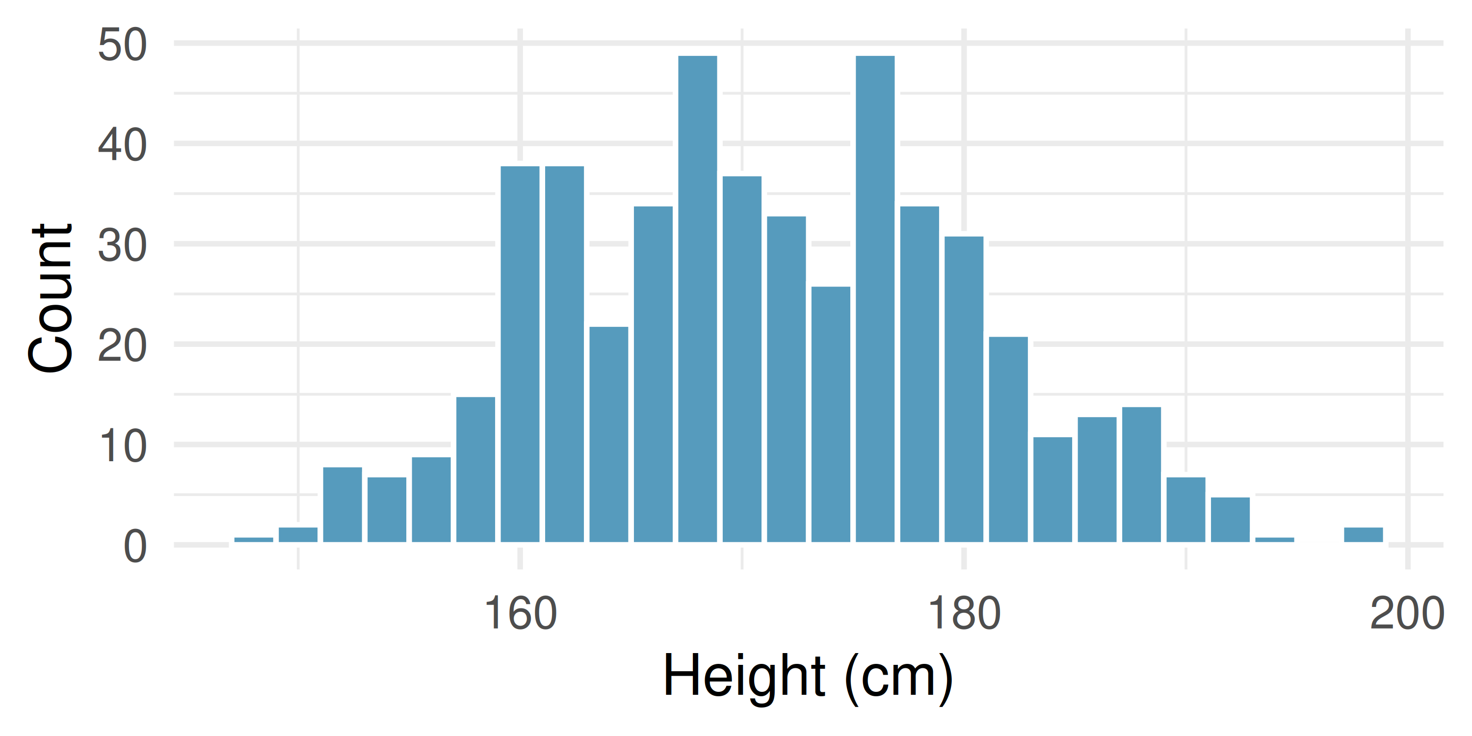
What are the point estimates for the average and median heights of active adults?
What are the point estimates for the standard deviation and IQR of heights of active adults?
Is a person who is 1m 80cm (180 cm) tall considered unusually tall? And is a person who is 1m 55cm (155cm) considered unusually short? Explain your reasoning.
The researchers take another random sample of physically active adults. Would you expect the mean and the standard deviation of this new sample to be the ones given above? Explain your reasoning.
The sample means obtained are point estimates for the mean height of all active individuals, if the sample of individuals is equivalent to a simple random sample. What measure do we use to quantify the variability of such an estimate? Compute this quantity using the data from the original sample under the condition that the data are a simple random sample.
- Heights of adults, standard error. Heights of 507 physically active adults have a mean of 171 cm and a standard deviation of 9.4 cm. Provide an estimate for the standard error of the mean for samples of following sizes. (Heinz et al. 2003)
n = 10
n = 50
n = 100
n = 1000
The standard error of the mean is a number which describes what?
- Heights of adults vs. kindergartners. Heights of 507 physically active adults have a mean of 171 cm and a standard deviation of 9.4 cm. (Heinz et al. 2003)
Would you expect the standard deviation of the heights of a few hundred kindergartners to be higher or lower than 9.4 cm? Explain your reasoning.
Suppose many samples of size 100 adults is taken and, separately, many samples of size 100 kindergarteners are taken. For each of the many samples, the average height is computed. Which set of sample averages would have a larger standard error of the mean, the adult sample averages or the kindergartner sample averages?
- Heights of adults, bootstrap interval. Researchers studying anthropometry collected body measurements, as well as age, weight, height and gender, for 507 physically active adults. The histogram below shows the sample distribution of bootstrapped means from 1,000 different bootstrap samples. (Heinz et al. 2003)
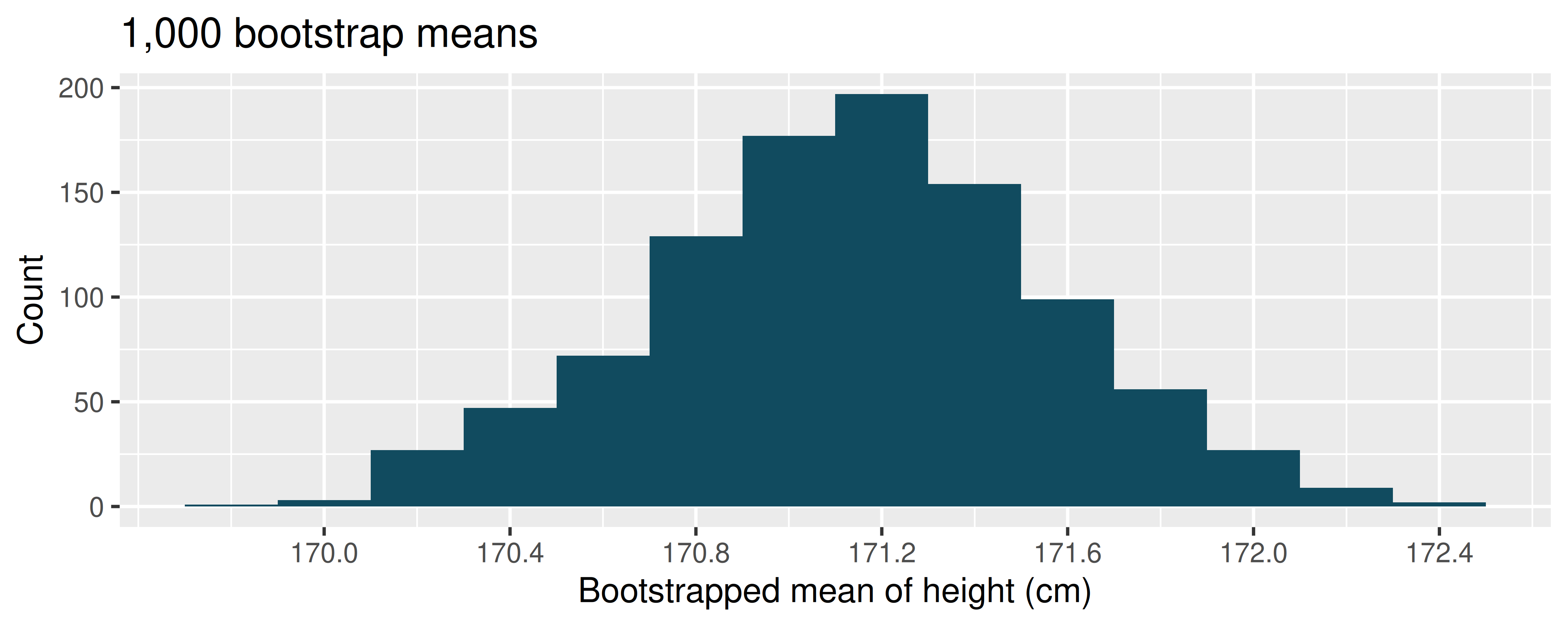
Given the bootstrap sampling distribution for the sample mean, find an approximate value for the standard error of the mean.
By looking at the bootstrap sampling distribution (1,000 bootstrap samples were taken), find an approximate 90% bootstrap percentile confidence interval for the true average adult height in the population from which the data were randomly sampled. Provide the interval as well as a one-sentence interpretation of the interval.
By looking at the bootstrap sampling distribution (1,000 bootstrap samples were taken), find an approximate 90% bootstrap SE confidence interval for the true average adult height in the population from which the data were randomly sampled. Provide the interval as well as a one-sentence interpretation of the interval.
- Identify the critical \(t\). A random sample is selected from an approximately normal population with unknown standard deviation. Find the degrees of freedom and the critical \(t\)-value (t\(^\star\)) for the given sample size and confidence level.
\(n = 6\), CL = 90%
\(n = 21\), CL = 98%
\(n = 29\), CL = 95%
\(n = 12\), CL = 99%
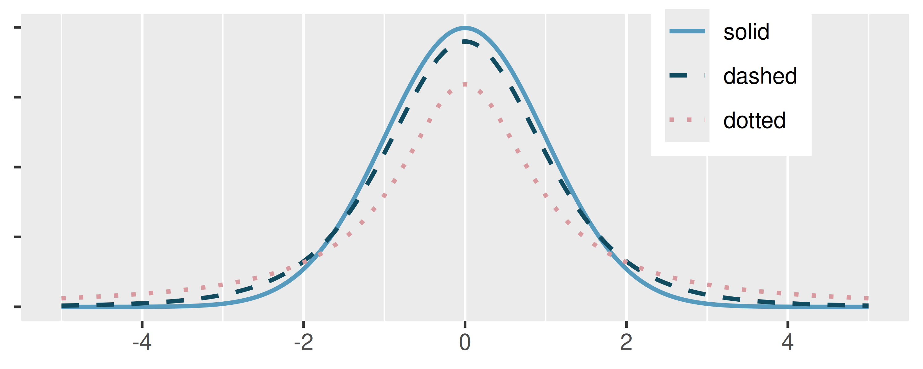
- \(t\)-distribution. The figure below shows three unimodal and symmetric curves: the standard normal (z) distribution, the \(t\)-distribution with 5 degrees of freedom, and the \(t\)-distribution with 1 degree of freedom. Determine which is which, and explain your reasoning.
- Length of gestation, confidence interval. Every year, the United States Department of Health and Human Services releases to the public a large dataset containing information on births recorded in the country. This dataset has been of interest to medical researchers who are studying the relation between habits and practices of expectant mothers and the birth of their children. In this exercise we work with a random sample of 1,000 cases from the dataset released in 2014. The length of pregnancy, measured in weeks, is commonly referred to as gestation. The histograms below show the distribution of lengths of gestation from the random sample of 1,000 births (on the left) and the distribution of bootstrapped means of gestation from 1,500 different bootstrap samples (on the right).
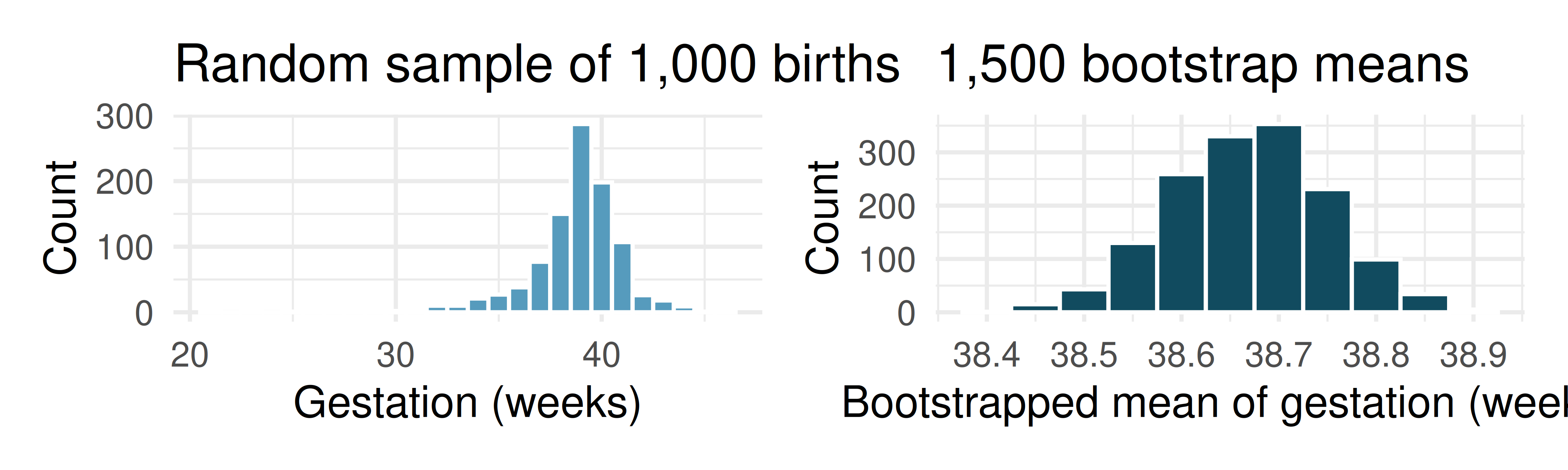
Given the bootstrap sampling distribution for the sample mean, find an approximate value for the standard error of the mean.
By looking at the bootstrap sampling distribution (1,500 bootstrap samples were taken), find an approximate 99% bootstrap percentile confidence interval for the true average gestation length in the population from which the data were randomly sampled. Provide the interval as well as a one-sentence interpretation of the interval.
By looking at the bootstrap sampling distribution (1,500 bootstrap samples were taken), find an approximate 99% bootstrap SE confidence interval for the true average gestation length in the population from which the data were randomly sampled. Provide the interval as well as a one-sentence interpretation of the interval.
- Interpreting confidence intervals for population mean. For each of the following statements, indicate if they are a true or false interpretation of the confidence interval. If false, provide a reason or correction to the misinterpretation. You collect a large sample and calculate a 95% confidence interval for the average number of cans of sodas consumed annually per adult in the US to be (440 cans, 520 cans), i.e., on average, adults in the US consume just under two cans of soda per day.
95% of adults in the US consume between 440 and 520 cans of soda per year.
There is a 95% probability that the true population average per adult yearly soda consumption is between 440 and 520 cans.
The true population average per adult yearly soda consumption is between 440 and 520 cans, with 95% confidence.
The average soda consumption of the people who were sampled is between 440 and 520 cans of soda per year, with 95% confidence.
- Working backwards, I. A 95% confidence interval for a population mean, \(\mu\), is given as (18.985, 21.015). The population distribution is approximately normal and the population standard deviation is unknown. This confidence interval is based on a simple random sample of 36 observations. Assuming that all conditions necessary for inference are satisfied, and using the \(t\)-distribution, calculate the sample mean, the margin of error, and the sample standard deviation.
- Working backwards, II. A 90% confidence interval for a population mean is (65, 77). The population distribution is approximately normal and the population standard deviation is unknown. This confidence interval is based on a simple random sample of 25 observations. Assuming that all conditions necessary for inference are satisfied, and using the \(t\)-distribution, calculate the sample mean, the margin of error, and the sample standard deviation.
- \(t^\star\) for the correct confidence level. As you’ve seen, the tails of a \(t-\)distribution are longer than the standard normal which results in \(t^{\star}_{df}\) being larger than \(z^{\star}\) for any given confidence level. When finding a CI for a population mean, explain how mistakenly using \(z^{\star}\) (instead of the correct \(t^{*}_{df}\)) would affect the confidence level.
- Possible bootstrap samples. Consider a simple random sample of the following observations: 47, 4, 92, 47, 12, 8. Which of the following could be a possible bootstrap samples from the observed data above? If the set of values could not be a bootstrap sample, indicate why not.
47, 47, 47, 47, 47, 47
92, 4, 13, 8, 47, 4
92, 47, 12
8, 47, 12, 12, 8, 4, 92
12, 4, 8, 8, 92, 12
- Fill in the blanks. We use a ___ to evaluate if data provide convincing evidence of a difference between two population means and we use a ___ to estimate this difference.
- Diamonds, bootstrap interval. We have data on two random samples of diamonds: 23 0.99 carat diamonds and 23 1 carat diamonds. Provided below is a histogram of bootstrap differences in means of price per carat of diamonds that weigh 0.99 carats and diamonds that weigh 1 carat. (Wickham 2016)
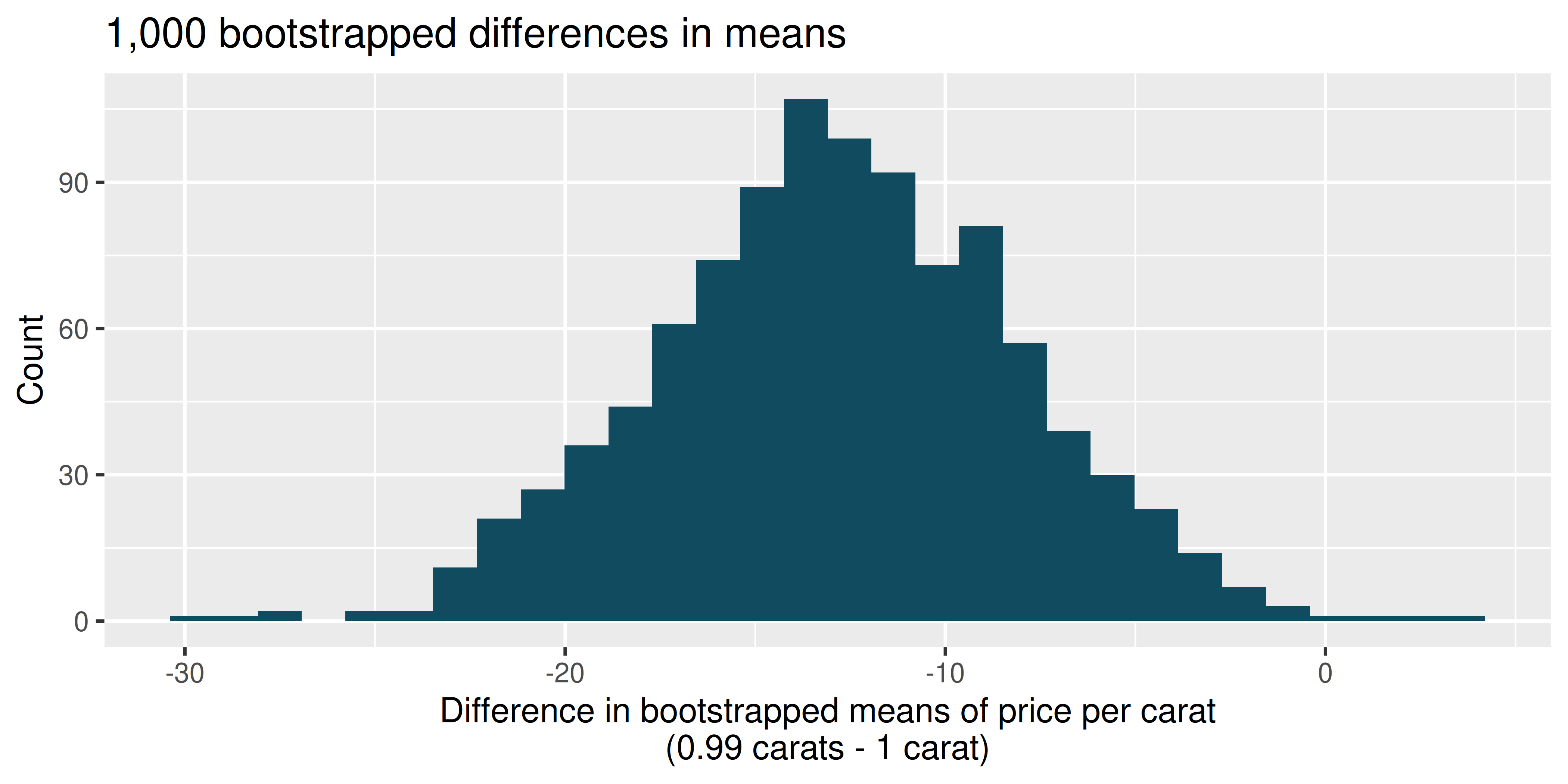
Using the bootstrap distribution, create a (rough) 95% bootstrap percentile confidence interval for the true population difference in prices per carat of diamonds that weigh 0.99 carats and 1 carat.
Using the bootstrap distribution, create a (rough) 95% bootstrap SE confidence interval for the true population difference in prices per carat of diamonds that weigh 0.99 carats and 1 carat. Note that the standard error of the bootstrap distribution is 4.64.
- Lizards running, bootstrap interval. We have data on top speeds (in m/sec) measured on a laboratory race track for two species of lizards: Western fence lizard (Sceloporus occidentalis) and Sagebrush lizard (Sceloporus graciosus). The bootstrap distribution below describes the variability of difference in means captured from 1,000 bootstrap samples of the lizard data. (Adolph 1987)
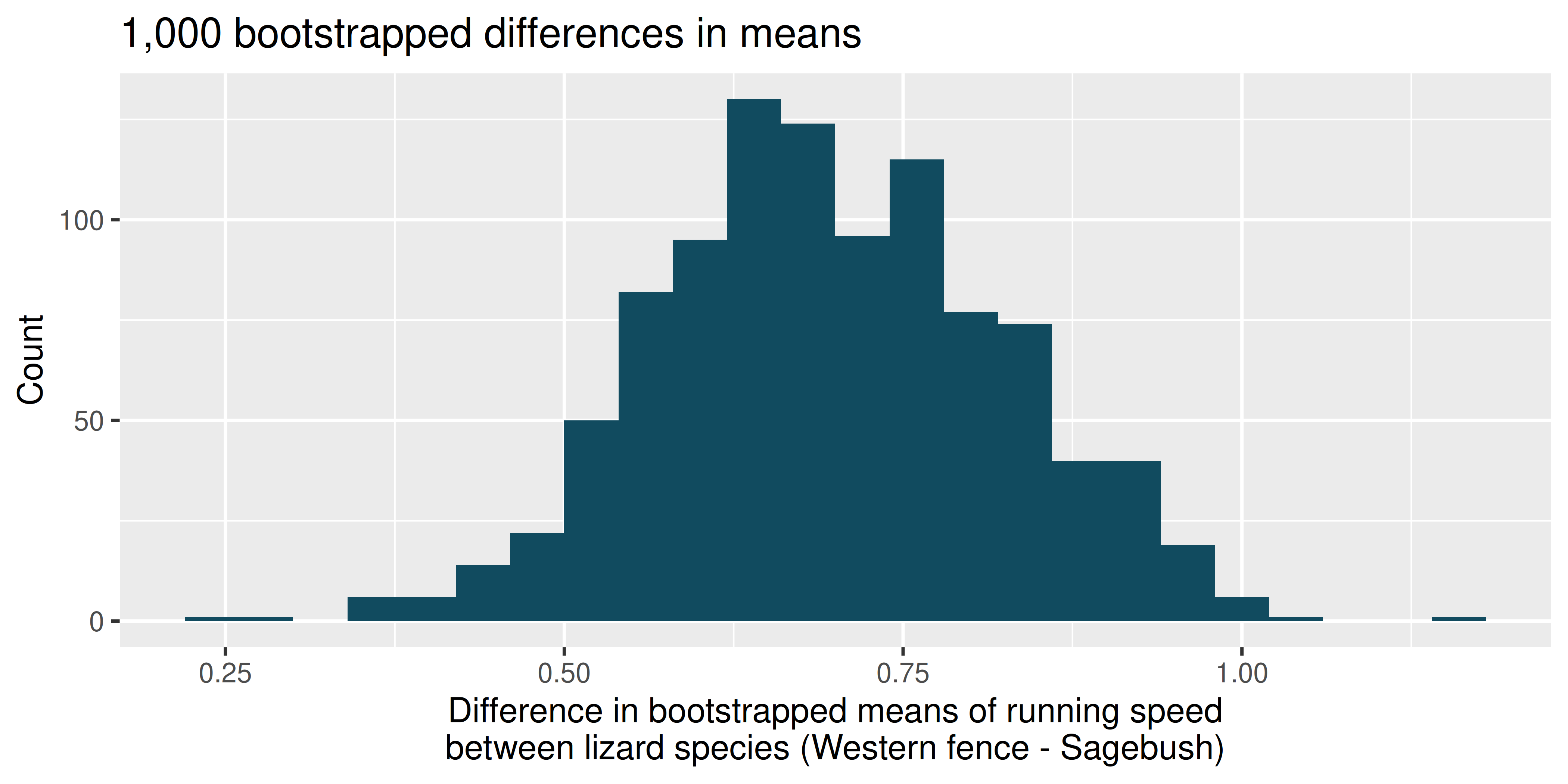
Using the bootstrap distribution, create a (rough) 90% percentile bootrap confidence interval for the true population difference in average speed of the Western fence lizard as compared with Sagebrush lizard.
Using the bootstrap distribution, create a (rough) 90% bootstrap SE confidence interval for the true population difference in average speed of the Western fence lizard as compared with Sagebrush lizard.
- Weight loss. You are reading an article in which the researchers have created a 95% confidence interval for the difference in average weight loss for two diets. They are 95% confident that the true difference in average weight loss over 6 months for the two diets is somewhere between (1 lb, 25 lbs). The authors claim that, “therefore diet A (\(\bar{x}_A\) = 20 lbs average loss) results in a much larger average weight loss as compared to diet B (\(\bar{x}_B\) = 7 lbs average loss).” Comment on the authors’ claim.
- Diamonds, mathematical interval. We have data on two random samples of diamonds: one with diamonds that weigh 0.99 carats and one with diamonds that weigh 1 carat. Each sample has 23 diamonds. Sample statistics for the price per carat of diamonds in each sample are provided below. Assuming that the conditions for conducting inference using a mathematical model are satisfied, construct a 95% confidence interval for the true population difference in prices per carat of diamonds that weigh 0.99 carats and 1 carat. (Wickham 2016)
| Mean | SD | n | |
|---|---|---|---|
| 0.99 carats | $44.51 | $13.32 | 23 |
| 1 carat | $57.20 | $18.19 | 23 |
- True / False: comparing means. Determine if the following statements are true or false, and explain your reasoning for statements you identify as false.
As the degrees of freedom increases, the \(t\)-distribution approaches normality.
If a 95% confidence interval for the difference between two population means contains 0, a 99% confidence interval calculated based on the same two samples will also contain 0.
If a 95% confidence interval for the difference between two population means contains 0, a 90% confidence interval calculated based on the same two samples will also contain 0.
- Difference of means. We collect two random samples from two different populations In each part below, consider the sample means \(\bar{x}_1\) and \(\bar{x}_2\) that we might observe from these two samples.
| Mean | Standard deviation | Sample size | |
|---|---|---|---|
| Population 1 | 15 | 20 | 50 |
| Population 2 | 20 | 10 | 30 |
What is the associated mean and standard deviation of \(\bar{x}_1\)?
What is the associated mean and standard deviation of \(\bar{x}_2\)?
Calculate and interpret the mean and standard deviation associated with the difference in sample means for the two groups, \(\bar{x}_2 - \bar{x}_1\).
How are the standard deviations from parts (a), (b), and (c) related?
- Air quality. Air quality measurements were collected in a random sample of 25 country capitals in 2013, and then again in the same cities in 2014. We would like to use these data to compare average air quality between the two years. Should we use a paired or non-paired test? Explain your reasoning.
- True / False: paired. Determine if the following statements are true or false. If false, explain.
In a paired analysis we first take the difference of each pair of observations, and then we do inference on these differences.
Two datasets of different sizes cannot be analyzed as paired data.
Consider two sets of data that are paired with each other. Each observation in one dataset has a natural correspondence with exactly one observation from the other dataset.
Consider two sets of data that are paired with each other. Each observation in one dataset is subtracted from the average of the other dataset’s observations.
- Paired or not? I. In each of the following scenarios, determine if the data are paired.
Compare pre- (beginning of semester) and post-test (end of semester) scores of students.
Assess gender-related salary gap by comparing salaries of randomly sampled men and women.
Compare artery thicknesses at the beginning of a study and after 2 years of taking Vitamin E for the same group of patients.
Assess effectiveness of a diet regimen by comparing the before and after weights of subjects.
- Paired or not? II. In each of the following scenarios, determine if the data are paired.
We would like to know if Intel’s stock and Southwest Airlines’ stock have similar rates of return. To find out, we take a random sample of 50 days, and record Intel’s and Southwest’s stock on those same days.
We randomly sample 50 items from Target stores and note the price for each. Then we visit Walmart and collect the price for each of those same 50 items.
A school board would like to determine whether there is a difference in average SAT scores for students at one high school versus another high school in the district. To check, they take a simple random sample of 100 students from each high school.
- Sample size and pairing. Determine if the following statement is true or false, and if false, explain your reasoning: If comparing means of two groups with equal sample sizes, always use a paired test.
- High School and Beyond, bootstrap interval. We considered the differences between the reading and writing scores of a random sample of 200 students who took the High School and Beyond Survey. The mean and standard deviation of the differences are \(\bar{x}_{read-write} = -0.545\) and \(s_{read-write}\) = 8.887 points. The bootstrap distribution below was produced by bootstrapping from the sample of differences in reading and writing scores 1,000 times.
Find an approximate 95% bootstrap percentile confidence interval for the true average difference in scores (read - write).
Find an approximate 95% bootstrap SE confidence interval for the true average difference in scores (read - write).
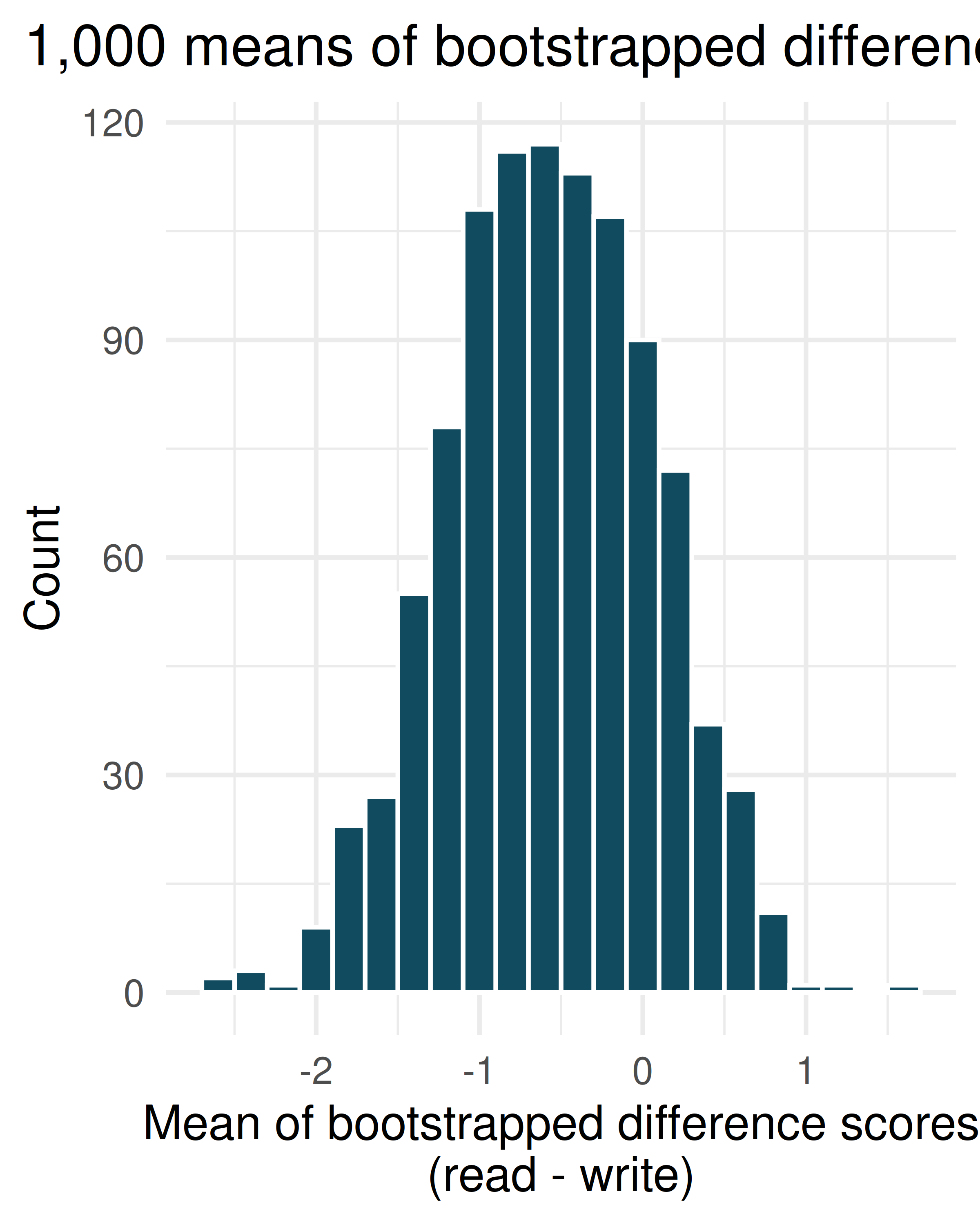
Interpret both confidence intervals using words like “population” and “score”.
From the confidence intervals calculated above, does it appear that there is a discernible difference in reading and writing scores, on average?
- Global warming, bootstrap interval. We considered the change in the 90\(^{th}\) percentile high temperature in 1950 versus 2022 at 26 sampled locations from the NOAA database. (NOAA 2023) The mean and standard deviation of the reported differences are 2.53\(^\circ\)F and 2.95\(^\circ\)F.
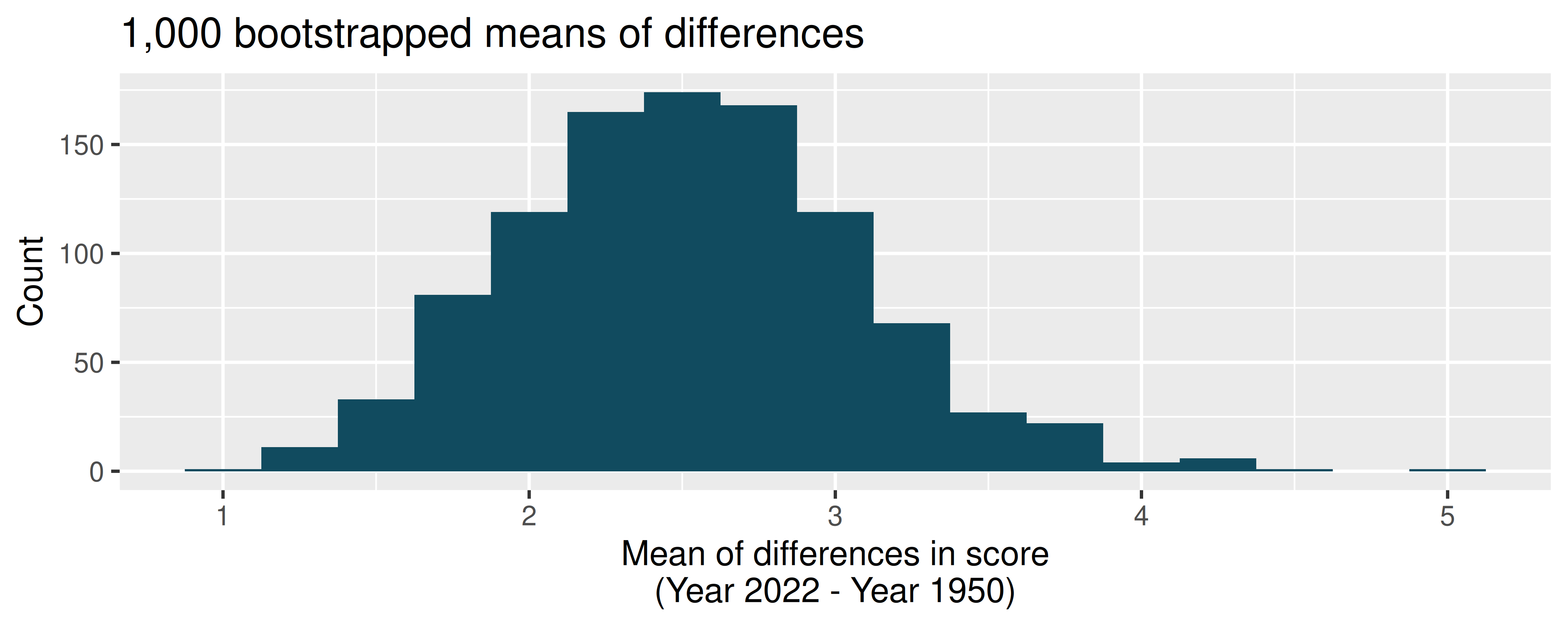
Calculate a 90% bootstrap percentile confidence interval for the average difference of 90\(^{th}\) percentile high temperature between 1950 and 2022.
Calculate a 90% bootstrap SE confidence interval for the average difference of 90\(^{th}\) percentile high temperature between 1950 and 2022.
Interpret both intervals in context.
Do the confidence intervals provide convincing evidence that there were hotter high temperatures in 2022 than in 1950 at NOAA stations? Explain your reasoning.
- High school and beyond, mathematical interval. We considered the differences between the reading and writing scores of a random sample of 200 students who took the High School and Beyond Survey. The mean and standard deviation of the differences are \(\bar{x}_{read-write} = -0.545\) and \(s_{read-write}\) = 8.887 points.
Calculate a 95% confidence interval for the average difference between the reading and writing scores of all students.
Interpret this interval in context.
Does the confidence interval provide convincing evidence that there is a real difference in the average scores? Explain.
- Global warming, mathematical interval. We considered the change in the 90\(^{th}\) percentile high temperature in 1950 versus 2022 at 26 sampled locations from the NOAA database. (NOAA 2023) The mean and standard deviation of the reported differences are 2.53\(^\circ\)F and 2.95\(^\circ\)F.
Calculate a 90% confidence interval for the average difference of 90\(^{th}\) percentile high temperature between 1950 and 2022. We’ve already checked the conditions for you.
Interpret the interval in context.
Does the confidence interval provide convincing evidence that there were hotter high temperatures in 2022 than in 1950 at NOAA stations? Explain your reasoning.
- Forest management. Forest rangers wanted to better understand the rate of growth for younger trees in the park. They took measurements of a random sample of 50 young trees in 2009 and again measured those same trees in 2019. The data below summarize their measurements, where the heights are in feet.
| Year | Mean | SD | n |
|---|---|---|---|
| 2009 | 12.0 | 3.5 | 50 |
| 2019 | 24.5 | 9.5 | 50 |
| Difference | 12.5 | 7.2 | 50 |
Construct a 99% confidence interval for the average growth of (what had been) younger trees in the park over 2009-2019.
StatLens Exercises
These exercises focus on the parts of inference a calculator can’t do for you: framing the question, choosing the right procedure, checking conditions, and interpreting what a tool reports. Where a link is given, let StatLens do the arithmetic and spend your effort on the reasoning.
Frame the question. A nutrition researcher wants to estimate the mean daily caffeine intake (in mg) among undergraduates at a large university. She collects a random sample of \(n = 48\) students and records each one’s daily intake.
- What is the parameter of interest? Describe it in words and give its symbol.
- Should the resulting confidence interval be one-sided or two-sided, and why?
- Why is the sample standard deviation \(s\) used in the \(t\)-procedure here, and not the population standard deviation \(\sigma\)?
Choose the procedure. For each scenario, name the procedure you would use — one-sample \(t\) (test or interval), two-sample \(t\) (independent groups), paired \(t\) (matched pairs), or not a means problem. You do not need to carry anything out; the skill here is matching the question to the method.
- Estimate the mean fuel economy (mpg) of a new car model from a sample of 25 test drives.
- Compare the mean recovery time of patients on Drug A vs. Drug B, where each patient was randomly assigned to one drug.
- Measure each runner’s 5K time before and after a 6-week training program; ask whether the program lowers times on average.
- Estimate the proportion of voters in a district who support a ballot measure.
- Compare the median household income in two counties.
Check conditions before you trust the interval. A small clinical study reports the resting heart rates of \(n = 12\) adults after an experimental intervention. Open the data in the One-Sample \(t\) tool (pick any small numeric dataset, or paste in a small sample of your own) and inspect the distribution.
- What two conditions does the one-sample \(t\)-interval require? State each in plain language.
- With only \(n = 12\), how would you decide whether the normality condition is reasonable? What feature of the dotplot or histogram would make you uneasy?
- If the histogram shows a clear right skew with one extreme outlier, is the \(t\)-interval still trustworthy? What would you do instead?
Run it and interpret it (two means). A study compared mean reaction times (ms) between a caffeinated group and a placebo group. Open a two-group dataset of your choice in the Two-Sample \(t\) tool.
Identify the explanatory and response variables, and define the parameter \(\mu_1 - \mu_2\) in words.
Run the tool. Report the 95% confidence interval for \(\mu_1 - \mu_2\). Does the interval contain 0?
Write a one-sentence conclusion in context, and say whether your confidence interval and a two-sided hypothesis test at \(\alpha = 0.05\) would lead to the same decision.
Which statement is the correct interpretation of the interval in (b)?
- There is a 95% probability that \(\mu_1 - \mu_2\) lies in this interval.
- If the experiment were repeated many times, about 95% of the intervals built this way would contain the true difference \(\mu_1 - \mu_2\).
- 95% of caffeinated participants fall within this interval.
Paired vs. independent — choose carefully, then compare. Twelve runners each ran a 5K race before and after a 6-week training program; you also have a separate sample of 12 different runners who did not train, run at the same point in the season.
- If you want to know whether the program lowered 5K times, why is the paired-sample analysis (on the within-runner differences) almost always more informative than treating the before-times and after-times as two independent groups?
- Open the Paired \(t\) tool with any paired dataset. Record the 95% CI for the mean difference. Then re-analyze the same numbers in the Two-Sample \(t\) tool as if they were independent groups. What is different about the standard error and the width of the CI?
- Now consider the untrained sample. To estimate the program’s effect against a no-training baseline, what would you compare, and which procedure would you use? Why is matching impossible here?
- A student says: “Paired is just a special case of two-sample.” Why is this misleading, even though both end up using the \(t\) distribution?
Compute-unit capstone — write conclusions across every procedure you have learned so far. By this point you have worked with the one-proportion \(z\), the two-proportion \(z\), the one-sample \(t\), the two-sample \(t\), and the paired \(t\). The last skill — taking a test result and writing what it means in context — is one that gets rusty quickly if you don’t practice across procedures.
Open Conclusion Practice — Compute scope. This link filters the scenario pool to just the five procedures from Part III (no chi-square, ANOVA, or regression — those come later). Each round gives you a randomized scenario with the test output already computed; your job is to assemble a formal conclusion (about the parameter, at the stated \(\alpha\)) and a practical conclusion (what a non-statistician stakeholder should take away). The tool scores you.
- Play at least 5 rounds. Aim for a passing score in each. Do you notice any pattern in the mistakes you make — do they cluster around a particular procedure, or a particular pitfall (misinterpreting p, misinterpreting the CI, over-claiming causation, etc.)?
- Which is harder for you: writing the formal conclusion, or writing the practical one? Why?
- Reflect: from the perspective of “what makes an inference class valuable,” which mattered more — computing p-values (which StatLens did for you) or writing correct conclusions (which you had to do)? What does this suggest about how you should split your study time going forward?
Adolph, S. C. 1987. “Physiological and Behavioral Ecology of the Lizards Sceloporus Occidentalis and Sceloporus Graciosus.” PhD thesis, University of Washington, Seattle, Washington.
Heinz, G., L. J. Peterson, R. W. Johnson, and C. J. Kerk. 2003. “Exploring Relationships in Body Dimensions.” Journal of Statistics Education 11 (2). http://www.openintro.org/redirect.php?go=textbook-body_dim_2003.
NOAA. 2023. “Climate Data Online.” http://www.openintro.org/redirect.php?go=textbook-noaa_1948_2018.
Wickham, H. 2016. ggplot2: Elegant Graphics for Data Analysis. Springer-Verlag New York. https://ggplot2.tidyverse.org.