18 Multiple Comparisons
When an ANOVA test rejects the null hypothesis, we know that at least one group mean differs from the others – but we do not know which groups differ. This chapter addresses the natural follow-up question: which specific pairs of groups have different means? Attempting many pairwise comparisons inflates the overall Type I error rate, so we need specialized methods that control for the fact that we are conducting multiple tests simultaneously. We introduce the multiple testing problem, the Bonferroni correction, and Tukey’s Honest Significant Difference (HSD) method.
See it in action. For the multiple-testing problem itself, work through the story-driven Do Green Jelly Beans Cause Acne? activity (family-wise error inflation, built around xkcd #882). For the actual post-hoc procedure, open Multiple Comparisons on any 3+ group numeric dataset — pairwise-CI table + forest plot, toggle Tukey HSD ↔︎ Bonferroni. Try insectsprays for the classic clean pattern.
18.1 The multiple testing problem
When we conduct a single hypothesis test at discernibility level \(\alpha = 0.05\), there is a 5% chance of incorrectly rejecting a true null hypothesis (a Type I error). But what happens when we conduct many tests?
Suppose we compare \(k = 4\) groups. How many pairwise comparisons are possible? If we conduct each test at \(\alpha = 0.05\) and all null hypotheses are actually true, what is the probability that we make at least one Type I error?
With 4 groups, there are \(\binom{4}{2} = 6\) pairwise comparisons. If we conduct each at \(\alpha = 0.05\), the probability that any single test does not produce a Type I error is \(1 - 0.05 = 0.95\). If the tests were independent, the probability that none of the 6 tests produces a Type I error would be:
\[P(\text{no errors}) = 0.95^6 = 0.735\]
So the probability of making at least one Type I error is:
\[P(\text{at least one error}) = 1 - 0.735 = 0.265\]
That is about a 27% chance of at least one false positive if the tests were independent. Pairwise comparisons are not actually independent – each group appears in several comparisons – so the true chance is somewhat lower (about 20% for all six comparisons among four groups), but it is still much higher than the 5% we intended.
18.1.1 Family-wise error rate
The probability of making at least one Type I error across all tests in a family of comparisons is called the family-wise error rate (FWER). When conducting \(m\) independent tests, each at discernibility level \(\alpha\), the FWER is:
\[\text{FWER} = 1 - (1 - \alpha)^m\]
The table below applies this independent-tests formula to all pairwise comparisons among \(k\) groups when \(\alpha = 0.05\):
| Number of groups (\(k\)) | Number of comparisons (\(m\)) | FWER from the independent-tests formula |
|---|---|---|
| 3 | 3 | 0.143 |
| 4 | 6 | 0.265 |
| 5 | 10 | 0.401 |
| 6 | 15 | 0.537 |
| 10 | 45 | 0.901 |
These values are an approximation. Pairwise comparisons share groups, so the tests are correlated, and the actual FWER for unadjusted pairwise \(t\)-tests is lower than the formula gives – roughly 0.12 for 3 groups and about 0.6 for 10 groups. Even so, with 10 groups we are more likely than not to make at least one Type I error if we use unadjusted pairwise tests. This is the core of the multiple comparisons problem: we need procedures that control the FWER at an acceptable level (typically 0.05).
Family-wise error rate (FWER).
The family-wise error rate is the probability of making one or more Type I errors among all the hypothesis tests in a family of comparisons. Methods like the Bonferroni correction and Tukey’s HSD are designed to keep the FWER at or below a specified level \(\alpha\).
18.2 The Bonferroni correction
The simplest method for controlling the family-wise error rate is the Bonferroni correction. The idea is straightforward: if we are conducting \(m\) tests and want the overall FWER to be at most \(\alpha\), we use a stricter discernibility level for each individual test.
Bonferroni correction.
When conducting \(m\) hypothesis tests and we want the family-wise error rate to be at most \(\alpha\), the Bonferroni correction uses an adjusted discernibility level for each individual test:
\[\alpha^* = \frac{\alpha}{m}\]
Equivalently, we can multiply each \(p\)-value by \(m\) (the adjusted \(p\)-value) and compare the result to the original \(\alpha\).
After an ANOVA with \(k = 4\) groups rejects \(H_0\), we want to conduct all pairwise comparisons at an overall \(\alpha = 0.05\). How many comparisons are there, and what adjusted discernibility level should we use for each?
There are \(\binom{4}{2} = 6\) pairwise comparisons. The Bonferroni-adjusted discernibility level is:
\[\alpha^* = \frac{0.05}{6} = 0.0083\]
So each individual two-sample \(t\)-test must have a \(p\)-value below 0.0083 to be considered discernible.
The Bonferroni correction is simple and broadly applicable – it can be used with any type of test, not just pairwise comparisons of means. However, it is conservative, meaning it may fail to detect real differences when they exist (higher Type II error). When the number of comparisons is very large, the Bonferroni correction can be overly strict.
18.2.1 Example: Exam scores
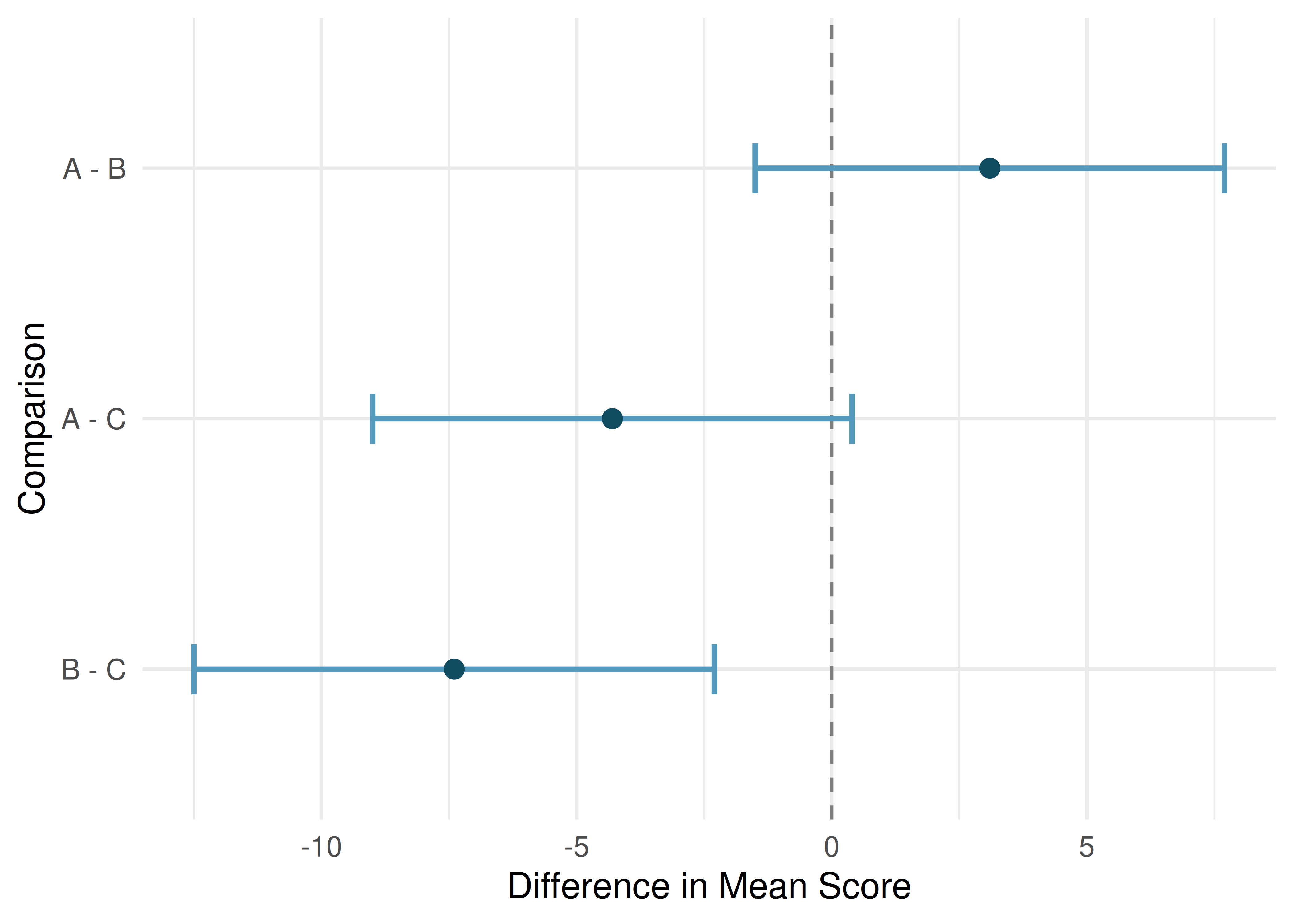
The ANOVA comparing the three exam versions (A, B, C) in the previous chapter gave \(F = 3.48\), with a \(p\)-value of 0.033 from the F-distribution. We rejected \(H_0\) and now want to know which exams differ.
With \(k = 3\) groups, there are \(\binom{3}{2} = 3\) pairwise comparisons. The Bonferroni-adjusted discernibility level is \(\alpha^* = 0.05/3 = 0.0167\).
Two-sample \(t\)-tests for the three pairs (using the pooled standard deviation from the ANOVA) give these \(p\)-values:
| Comparison | \(p\)-value | Discernible at \(\alpha^* = 0.0167\)? |
|---|---|---|
| A vs. B | 0.222 | No |
| A vs. C | 0.144 | No |
| B vs. C | 0.009 | Yes |
Only the comparison between exams B and C is discernible after the Bonferroni correction. We conclude that there is evidence of a difference in difficulty between exams B and C, but we cannot say the other pairs differ.
18.3 Tukey’s Honest Significant Difference
A more powerful alternative to the Bonferroni correction for pairwise comparisons of means is Tukey’s Honest Significant Difference (HSD) method. While the Bonferroni correction is general-purpose, Tukey’s method is specifically designed for comparing all pairs of group means after ANOVA, and it is less conservative.
18.3.1 How Tukey’s HSD works
Tukey’s HSD computes a single critical difference – the minimum difference between two group means that would be considered statistically discernible. The procedure uses the Studentized range distribution to determine this critical value.
For each pair of groups \(j\) and \(j'\), the test statistic is:
\[q = \frac{\bar{x}_j - \bar{x}_{j'}}{\sqrt{MSE / n^*}}\]
where \(MSE\) is the mean square error from the ANOVA, and \(n^*\) is a measure of the group sample size (when group sizes are equal, \(n^* = n_j\); when unequal, a harmonic mean is often used). The statistic \(q\) is compared to critical values from the Studentized range distribution.
Tukey’s HSD.
Tukey’s Honest Significant Difference method controls the family-wise error rate at \(\alpha\) when making all pairwise comparisons of group means. It computes a confidence interval for each pairwise difference:
\[(\bar{x}_j - \bar{x}_{j'}) \pm q^* \cdot \sqrt{\frac{MSE}{n^*}}\]
where \(q^*\) is the critical value from the Studentized range distribution with \(k\) groups and \(n - k\) degrees of freedom. If the confidence interval does not contain zero, the difference is discernible.
18.3.2 Example: MLB batting positions
After the ANOVA for MLB batting data (\(F = 5.077\), \(p = 0.0066\)), we rejected \(H_0\) and want to identify which position pairs differ in on-base percentage. Tukey’s HSD produces the following pairwise comparisons:
| Comparison | Difference | 95% CI | Discernible? |
|---|---|---|---|
| IF - OF | -0.001 | (-0.011, 0.008) | No |
| C - OF | -0.018 | (-0.032, -0.004) | Yes |
| C - IF | -0.016 | (-0.030, -0.003) | Yes |
Catchers have a discernibly lower mean on-base percentage than both outfielders and infielders: neither the C − OF interval nor the C − IF interval contains zero, even after Tukey’s adjustment for making three comparisons. The difference between infielders and outfielders is not discernible – its interval comfortably includes zero. So the discernible ANOVA result is driven by catchers, whose average OBP is roughly 0.016 to 0.018 lower than that of the other two positions.
18.4 Interpreting post-hoc results
Post-hoc tests (like Bonferroni or Tukey’s HSD) are typically conducted after a discernible ANOVA result. Several important principles guide their interpretation:
18.4.1 When to use post-hoc tests
A common convention is to conduct post-hoc pairwise comparisons only after ANOVA rejects the null hypothesis. If the ANOVA \(p\)-value is not discernible, many analysts treat hunting through pairwise differences as a form of data snooping. This is a convention rather than a strict requirement: Tukey’s HSD controls the family-wise error rate on its own, whether or not an ANOVA is run first.
18.4.2 Reporting results
When reporting results of multiple comparisons, it is common to use compact letter displays. Groups that share a letter are not discernibly different from each other:
| Group | Mean | Grouping |
|---|---|---|
| A | 75.1 | ab |
| B | 72.0 | a |
| C | 78.9 | b |
In this notation, Groups A and B share the letter “a”, so they are not discernibly different, and Groups A and C share the letter “b”, so they are not discernibly different either. Groups B and C share no letter, so they are discernibly different. Group A, sharing a letter with both B and C, is not discernibly different from either.
18.4.3 Confidence intervals for differences
An especially useful way to present multiple comparison results is through confidence intervals for pairwise differences. If a confidence interval contains zero, the two groups are not discernibly different. If the interval is entirely positive or entirely negative, the groups differ.
18.4.4 Common mistakes
Running multiple pairwise tests without correction. This inflates the Type I error rate. Always use a correction method when conducting multiple comparisons.
Hunting for pairwise differences after a non-discernible ANOVA. By common convention, if the overall \(F\)-test does not reject \(H_0\), we do not go looking for pairwise differences. If you do examine them, use a method such as Tukey’s HSD that controls the family-wise error rate, and report the results as exploratory.
Ignoring practical importance. A statistically discernible difference may be too small to matter in practice. Always consider the magnitude of the differences, not just the \(p\)-values.
Over-interpreting non-discernible pairwise comparisons. A non-discernible pairwise comparison after a discernible ANOVA does not mean the groups are equal – it means we do not have enough evidence to declare them different individually.
18.5 Bonferroni vs. Tukey: When to use which
Both methods control the family-wise error rate, but they have different strengths:
| Feature | Bonferroni | Tukey’s HSD |
|---|---|---|
| Generality | Any set of tests | Pairwise comparisons of means only |
| Power | More conservative (less powerful) | Less conservative (more powerful) |
| Assumptions | None beyond the individual tests | Equal group variances (same as ANOVA) |
| Best for | Small number of planned comparisons | All pairwise comparisons after ANOVA |
Rule of thumb: If you are comparing all pairs of group means after a discernible ANOVA, use Tukey’s HSD. If you have a small number of pre-planned comparisons (not necessarily all pairs), the Bonferroni correction is appropriate.
18.6 Chapter review
18.6.1 Summary
When ANOVA rejects the null hypothesis, the natural follow-up question is: which groups differ? Performing many pairwise tests without correction inflates the family-wise error rate, making false positives likely. The Bonferroni correction divides the discernibility level by the number of comparisons, which is simple but conservative. Tukey’s HSD method is specifically designed for all pairwise comparisons of means after ANOVA and is typically more powerful. Both methods control the family-wise error rate at the desired level.
18.6.2 Key terms
- Multiple comparisons problem
- Family-wise error rate (FWER)
- Bonferroni correction
- Tukey’s Honest Significant Difference (HSD)
- Post-hoc test
- Compact letter display
18.7 Exercises
Answers to odd-numbered exercises are provided in the Exercise Solutions appendix at the back of the book.
- True / False: ANOVA, I. Determine if the following statements are true or false in ANOVA, and explain your reasoning for statements you identify as false.
As the number of groups increases, the modified discernibility level for pairwise tests increases as well.
As the total sample size increases, the degrees of freedom for the residuals increases as well.
The constant variance condition can be somewhat relaxed when the sample sizes are relatively consistent across groups.
The independence assumption can be relaxed when the total sample size is large.
- True / False: ANOVA, II. Determine if the following statements are true or false, and explain your reasoning for statements you identify as false.
If the null hypothesis that the means of four groups are all the same is rejected using ANOVA at a 5% discernibility level, then…
we can then conclude that all the means are different from one another.
the standardized variability between groups is higher than the standardized variability within groups.
the pairwise analysis will identify at least one pair of means that are discernibly different.
the appropriate \(\alpha\) to be used in pairwise comparisons is 0.05 / 4 = 0.0125 since there are four groups.
StatLens Exercises
Let StatLens do the arithmetic; spend your effort on the reasoning a calculator can’t do.
Frame the problem. A researcher measures reaction time under five different lighting conditions and wants to know which conditions produce different mean reaction times. She plans to run all \(\binom{5}{2} = 10\) pairwise \(t\)-tests, each at \(\alpha = 0.05\).
- What is the per-test Type I error rate? What is the family-wise Type I error rate, and how do they differ?
- Under the assumption that all 10 null hypotheses are true and the tests are independent, what is the probability of at least one false positive across the 10 tests?
- A colleague suggests: “Just report the per-test \(\alpha\); don’t worry about the family-wise rate.” Why is that unacceptable when the goal is to identify which conditions differ?
Choose the procedure. For each scenario, name the appropriate approach — Tukey HSD, Bonferroni, just the ANOVA F-test (no post-hoc needed), or not a multiple-comparisons problem.
- ANOVA rejects \(H_0\) across 4 fertilizer brands; you want to identify which brands differ from which.
- ANOVA fails to reject \(H_0\) across 4 fertilizer brands.
- You have 3 groups but pre-specified only two comparisons of interest before seeing the data (e.g., new-treatment vs. control, and new-treatment vs. standard).
- You want to compare mean scores across two teaching methods.
- You want to test the same difference-in-means for 100 different genes to see which are associated with a disease.
Check conditions before you trust the post-hoc. Open the Multiple Comparisons tool loaded with the classic
insectspraysdata (6 insecticides, count of insects found on each treated plot).- Confirm from the tool’s display: how many groups? What is the smallest per-group \(n\)? Is that enough for the pairwise procedure to work?
- What conditions does the Tukey HSD test require, beyond just “3+ groups”?
- The tool’s output shows the ANOVA table above the pairwise panel. Why is it appropriate to inspect the omnibus F-test first, even if you plan to do pairwise comparisons?
Run it and interpret it. Stay in the Multiple Comparisons tool. Make sure
?posthoc=tukeyis active.- Report the omnibus \(F\) statistic and p-value. Does the ANOVA reject \(H_0\)?
- In the pairwise table, count how many pairs have adjusted p-values below 0.05. How many pairs are declared not discernibly different?
- Read the forest plot: which pairs’ CIs cross zero, and which do not? Group the 6 sprays into “equivalence classes” (letters that don’t discernibly differ from each other but do differ from other classes).
- A student writes: “Sprays A and B differ from Spray C at family-wise \(\alpha = 0.05\).” Write the correct sentence including which quantity has family-wise coverage, and what “family-wise” actually means for the interpretation.
- The tool warns not to run post-hoc if the omnibus F is not significant. Why?
Bonferroni vs. Tukey — when do they agree? Switch the tool between
?posthoc=tukeyand?posthoc=bonferroni(or use the toggle).- Compare the widths of the pairwise 95% CIs under Tukey vs. Bonferroni on the
insectspraysdata. Which method gives narrower intervals? - Repeat on a smaller dataset (e.g., 3 groups, small \(n\)). Do the two methods still favor Tukey by the same margin?
- Why does Tukey give tighter intervals than Bonferroni when the goal is all pairwise comparisons of means? Tie your answer to what each method is actually controlling.
- When would you prefer Bonferroni over Tukey?
- A student is confused because on one dataset Bonferroni declares an extra pair discernibly different that Tukey does not. What could explain that, and which conclusion should you trust?
- Compare the widths of the pairwise 95% CIs under Tukey vs. Bonferroni on the