29 Type II Error and Power
In the chapter on decision errors we met the two ways a hypothesis test can go wrong and named their probabilities \(\alpha\) and \(\beta\). The Type I error rate \(\alpha\) is ours to choose; the Type II error rate \(\beta\) is not — it depends on the unknown truth. This chapter takes a closer look at \(\beta\): we use simulation to see how often a real effect goes undetected, examine the factors that drive the Type II error rate, and connect these ideas to the power of a study. This material extends beyond the core STAT 145 sequence and is intended for readers who want to go deeper.
29.1 Recap: the two error types
Recall from the chapter on decision errors:
- A Type I error rejects a true \(H_0\); its probability is the discernibility level \(\alpha\), which we choose.
- A Type II error fails to reject \(H_0\) when \(H_A\) is true; its probability is \(\beta\).
We can set \(\alpha\) directly, but \(\beta\) depends on the effect size, the sample size, and the variability in the data. The rest of this chapter studies what determines \(\beta\) — and how to drive it down.
29.2 Visualizing Type II error
The most effective way to build intuition about Type II error is to think about what happens when there is a real effect but our test fails to detect it. Simulation makes this concrete.
29.2.1 A simulation thought experiment
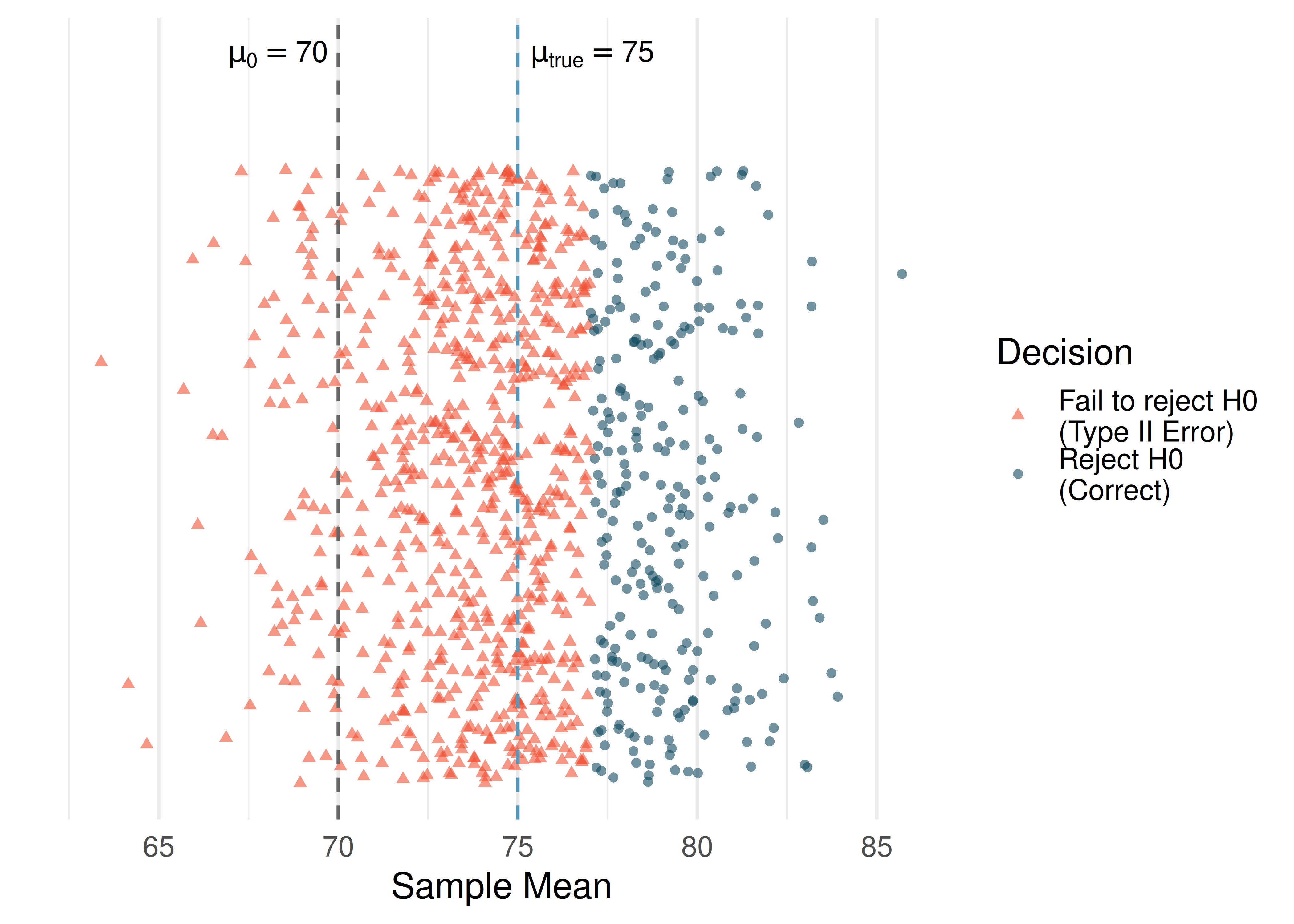
Imagine the following scenario. A tutoring program truly raises students’ exam scores by an average of 5 points (on a 100-point scale). The standard deviation of exam scores in the population is 15 points. A researcher recruits \(n = 20\) students, has them go through the tutoring program, and compares their scores to the known population mean using a one-sided one-sample \(t\)-test (\(H_A: \mu > 70\)) at \(\alpha = 0.05\).
Here is what might happen:
- The truth: \(\mu = 75\) (population mean with tutoring), while \(\mu_0 = 70\) (the null hypothesis value without tutoring). The real effect is \(\mu - \mu_0 = 5\) points.
- One simulated study: The researcher collects 20 scores. Due to natural variability, the sample mean might be \(\bar{x} = 73.2\) with \(s = 14.8\). The test statistic is:
\[t = \frac{73.2 - 70}{14.8 / \sqrt{20}} = \frac{3.2}{3.31} = 0.97\]
The \(p\)-value for this test is about 0.17 — not discernible at \(\alpha = 0.05\). The researcher fails to reject \(H_0\), even though the tutoring program really does work. This is a Type II error.
- Another simulated study: A different random sample of 20 students happens to include several who benefited greatly from tutoring. The sample mean is \(\bar{x} = 76.8\) with \(s = 13.5\). Now:
\[t = \frac{76.8 - 70}{13.5 / \sqrt{20}} = \frac{6.8}{3.02} = 2.25\]
The \(p\)-value is about 0.018 — discernible at \(\alpha = 0.05\). This time the researcher correctly rejects \(H_0\). This is a correct decision.
29.2.2 What happens across many studies?
If we repeated this experiment 1,000 times — each time drawing a fresh sample of 20 students from a population where the true effect is 5 points — we would find that roughly 400 of those experiments reject \(H_0\) and roughly 600 do not. That means:
- About 40% of the time, we correctly detect the real effect.
- About 60% of the time, we commit a Type II error.
The Type II error rate is \(\beta \approx 0.60\) — alarmingly high! About three in five studies with this design would miss the real effect. This is not because the effect doesn’t exist; it’s because the sample size is too small relative to the effect size and variability.
In the tutoring program simulation above, what would happen to the Type II error rate if the researcher increased the sample size from 20 to 100 students? Would \(\beta\) increase, decrease, or stay the same?
Show answer
The Type II error rate would decrease substantially. With 100 students instead of 20, the standard error drops from \(15/\sqrt{20} = 3.35\) to \(15/\sqrt{100} = 1.50\). The test becomes much more precise, making it easier to distinguish the true mean of 75 from the null value of 70. In fact, with \(n = 100\), the power would be about 95%, meaning \(\beta \approx 0.05\) — the test would miss the real effect only about 5% of the time.See it in action. Open the Power & Error Visualizer to see Type II error: it overlays the null and alternative curves and shades \(\alpha\), \(\beta\), and the power \(1-\beta\). Increase sample size or effect size and watch \(\beta\) shrink; lower \(\alpha\) and watch it grow. For the sim companion, pair with the Power Lab (repeated z-tests, empirical reject-rate).
29.3 Factors that affect the Type II error rate
Four key factors determine how likely a study is to commit a Type II error:
29.3.1 1. Effect size
The effect size is the magnitude of the difference between the true parameter value and the null hypothesis value. Larger effects are easier to detect.
- If a tutoring program raises scores by 20 points, almost any reasonable study will detect it.
- If a tutoring program raises scores by 2 points, you need a very large or very precise study to detect it.
Intuitively, a large effect “sticks out” from the noise, while a small effect can easily be hidden by random variability.
29.3.2 2. Sample size
Larger samples provide more precise estimates and smaller standard errors. The standard error of the sample mean is \(SE = \sigma / \sqrt{n}\), which decreases as \(n\) increases. A smaller standard error means the sampling distribution is narrower, making it easier to distinguish the true effect from zero.
More data, fewer missed effects. Increasing the sample size is the most common way to reduce the Type II error rate. This is why large clinical trials with thousands of participants are more likely to detect treatment effects than small pilot studies.
29.3.3 3. Population variability (\(\sigma\))
When individual observations are highly variable, it is harder to estimate the population mean precisely. The standard error depends directly on \(\sigma\): high variability means a wide sampling distribution, which makes it harder to distinguish \(H_A\) from \(H_0\).
For example, if exam scores range from 20 to 100 with \(\sigma = 25\), it is much harder to detect a 5-point effect than if scores range from 60 to 80 with \(\sigma = 5\).
A researcher is studying whether a dietary supplement improves reaction time. She can either recruit participants from the general population (where reaction times are highly variable) or from a group of trained athletes (where reaction times are more consistent). Which group would give her study a lower Type II error rate, assuming the supplement has the same true effect in both populations?
Show answer
The group of trained athletes would give a lower Type II error rate because their reaction times are less variable (smaller \(\sigma\)). A smaller \(\sigma\) leads to a smaller standard error, making it easier to detect the true effect of the supplement.29.3.4 4. Discernibility level (\(\alpha\))
As we discussed in Section 8.5, a smaller \(\alpha\) makes the test more conservative — it demands stronger evidence before rejecting \(H_0\). This directly increases \(\beta\) because the rejection region shrinks.
The table below summarizes these four factors:
| Factor | Change | Effect on \(\beta\) |
|---|---|---|
| Effect size | Larger effect | \(\beta\) decreases |
| Sample size (\(n\)) | Larger \(n\) | \(\beta\) decreases |
| Population variability (\(\sigma\)) | Larger \(\sigma\) | \(\beta\) increases |
| Discernibility level (\(\alpha\)) | Smaller \(\alpha\) | \(\beta\) increases |
A researcher plans a two-sample \(t\)-test to compare a new therapy to a standard therapy. She knows from pilot data that the standard deviation of patient outcomes is about \(\sigma = 12\). She is hoping to detect a difference of at least 4 points between the two therapies. Her initial plan calls for 30 patients per group with \(\alpha = 0.05\).
The standard error for the difference in means is approximately:
\[SE = \sqrt{\frac{12^2}{30} + \frac{12^2}{30}} = \sqrt{\frac{144}{30} + \frac{144}{30}} = \sqrt{9.6} = 3.10\]
The rejection boundary for a two-sided test is approximately \(1.96 \times SE = 1.96 \times 3.10 = 6.07\). Since the true effect is only 4 points — smaller than the rejection boundary of 6.07 — the study will more often than not fail to detect the effect. The Type II error rate will be high.
What could she change to reduce the Type II error rate?
She has several options: (1) increase the sample size to reduce the standard error, (2) try to reduce variability through better measurement or a more homogeneous study population, or (3) increase \(\alpha\) to 0.10 (though this increases the Type I error rate). The most practical option is usually to increase the sample size.
29.4 Practical vs. statistical discernibility revisited
The concepts of Type I and Type II error are closely connected to the distinction between statistical discernibility and practical importance that we first encountered in earlier chapters.
Statistical discernibility means the data provide enough evidence to reject \(H_0\) at our chosen \(\alpha\) level. It says: “The effect is probably not zero.”
Practical importance means the effect is large enough to matter in the real world. It says: “The effect is big enough to be useful.”
These are different questions, and they can give different answers:
| Scenario | Statistically discernible? | Practically important? | What happened? |
|---|---|---|---|
| Large effect, large \(n\) | Yes | Yes | Ideal outcome |
| Large effect, small \(n\) | Possibly not | Yes | Type II error risk — effect exists but may be missed |
| Small effect, large \(n\) | Yes | No | “Discernible but trivial” — very large studies can detect tiny, unimportant effects |
| Small effect, small \(n\) | No | No | No news |
The second row (large effect, small \(n\)) is the Type II error danger zone: a real, important effect exists, but the study is too small to detect it. The third row (small effect, large \(n\)) represents a different problem: a large study that detects a trivially small effect that has no practical importance.
A study with 50,000 participants finds that a new teaching method raises test scores by 0.3 points on a 100-point scale, with \(p = 0.002\). Is this result practically important?
The result is statistically discernible (\(p = 0.002 < 0.05\)), meaning we have strong evidence that the effect is not zero. However, a 0.3-point improvement on a 100-point scale is almost certainly too small to matter in practice. No school would adopt a new teaching method for a gain of one-third of a point. This is a case of statistical discernibility without practical importance — the study was so large that it detected a real but trivially small effect.
Statistical discernibility is not the same as practical importance. A statistically discernible result tells you the effect is probably real, but it does not tell you the effect is important. Always consider the size of the effect, not just whether it is statistically discernible.
A small pilot study with 12 participants finds that a new exercise program reduces resting heart rate by 8 beats per minute, but the result is not statistically discernible (\(p = 0.09\)). Does this mean the exercise program doesn’t work?
Show answer
Not necessarily. An 8 bpm reduction in resting heart rate is a clinically meaningful effect. The study may simply have been too small to detect it — this is a potential Type II error. The non-discernible result means we don’t have enough evidence to be confident the effect is real, but it doesn’t prove the program is ineffective. A larger study with more participants would be warranted.29.5 Chapter review
29.5.1 Summary
This chapter looked closely at the Type II error rate \(\beta\) and the power of a test. Simulation shows that a study with a small sample, a small true effect, or high variability can fail to detect a real effect a large fraction of the time. Four factors govern \(\beta\): the effect size (larger effects are easier to detect), the sample size (more data lowers \(\beta\)), the population variability (more variability raises \(\beta\)), and the discernibility level (a smaller \(\alpha\) raises \(\beta\)). Finally, statistical discernibility and practical importance are not the same: a very large study can detect a trivially small effect, while a small study can miss an important one.
29.6 Exercises
Answers to odd-numbered exercises are provided in the Exercise Solutions appendix at the back of the book.
- Which is higher? In each part below, there is a value of interest and two scenarios: (i) and (ii). For each part, report if the value of interest is larger under scenario (i), scenario (ii), or whether the value is equal under the scenarios.
The standard error of \(\hat{p}\) when (i) \(n = 125\) or (ii) \(n = 500\).
The margin of error of a confidence interval when the confidence level is (i) 90% or (ii) 80%.
The p-value for a Z-statistic of 2.5 calculated based on a (i) sample with \(n = 500\) or based on a (ii) sample with \(n = 1000\).
The probability of making a Type II error when the alternative hypothesis is true and the discernibility level is (i) 0.05 or (ii) 0.10.
- Same observation, different sample size. Suppose you conduct a hypothesis test based on a sample where the sample size is \(n = 50\), and arrive at a p-value of 0.08. You then refer back to your notes and discover that you made a careless mistake, the sample size should have been \(n = 500\). Will your p-value increase, decrease, or stay the same? Explain.
- Practical importance vs. statistical discernibility. Determine whether the following statement is true or false, and explain your reasoning: “With large sample sizes, even small differences between the null value and the observed point estimate can be statistically discernible.”
StatLens Exercises
Let StatLens do the arithmetic; spend your effort on the reasoning a calculator can’t do.
See \(\beta\) on the dual-curve picture. Open the Power & Error Visualizer.
- Where on the picture is \(\beta\) shaded? Why does it live under the alternative curve, not the null?
- Read the value of \(\beta\). What does “\(\beta = 0.14\)” mean in plain English for an experiment at these settings?
- Now decrease \(\delta\) to 0.5 (smaller effect). What happens to \(\beta\)? Why?
- Reset and decrease \(\sigma\) to 1 (less noise). What happens to \(\beta\)? Why?
Simulating Type II errors. Open the Power Lab (simulation).
- Run 500 simulated \(z\)-tests at these settings. The empirical reject rate is the simulated power. What’s the simulated \(\beta = 1 -\) power?
- In the hit/miss/false-alarm strip, what colour represents Type II errors? Roughly what fraction of dots are that colour?
- Increase \(n\) to 200 and re-run. Does \(\beta\) shrink as expected?
- A researcher says: “I’ll just call \(\beta\) small because my \(\alpha\) is small.” Why is this wrong?
When is “no evidence” no evidence? A trial of \(n = 30\) patients tests a new treatment with \(H_0: \mu = 0\) vs. \(H_A: \mu > 0\) at \(\alpha = 0.05\). The result: p = 0.18, “no discernible effect.”
- Using the Power & Error Visualizer (preset to \(\delta = 0.3, \sigma = 1\)), compute the power if the true effect were \(\delta = 0.3\). Is that high enough to call “no detected effect” informative?
- What if the true effect were \(\delta = 1\)? Re-check with the tool.
- Explain in one sentence the difference between “no evidence of effect” and “evidence of no effect.”
- What sentence should actually appear in the trial’s discussion section, given the modest power?