30  Statistical Power

Extended Content. This chapter extends beyond UWL’s core STAT 145 curriculum. It is included for completeness and for instructors who wish to cover additional topics. Content is in draft form.

In the Type II error and power chapter, we saw that a hypothesis test can miss a real effect — a Type II error. The flip side of this coin is power: the probability that a test correctly detects a real effect. Power is not just a theoretical concept; it is the foundation of good study design. Before collecting data, researchers need to ask: “Is my study large enough to find the effect I’m looking for?” This chapter defines power, explores the factors that influence it, and shows how simulation can estimate power when formulas are unavailable.

30.1 What is power?

In the Type II error and power chapter, we defined the Type II error rate \(\beta\) as the probability of failing to reject \(H_0\) when \(H_A\) is true. Power is simply the complement of \(\beta\).

The power of a hypothesis test is the probability of rejecting the null hypothesis when the alternative hypothesis is true:

\[\text{Power} = 1 - \beta = P(\text{reject } H_0 \mid H_A \text{ is true})\]

Power answers the question: “If there is a real effect, how likely is my study to detect it?”

The four possible outcomes of a hypothesis test, with their probabilities, are:

Table 30.1: Probabilities of each outcome in a hypothesis test.

	\(H_0\) is true	\(H_A\) is true
Reject \(H_0\)	\(\alpha\) (Type I error)	\(1 - \beta\) (Power)
Fail to reject \(H_0\)	\(1 - \alpha\) (Correct)	\(\beta\) (Type II error)

Notice the two columns must each sum to 1:

• When \(H_0\) is true: \(\alpha + (1 - \alpha) = 1\)
• When \(H_A\) is true: \((1 - \beta) + \beta = 1\)

Power = 1 − \(\beta\). A test with high power (close to 1) is very likely to detect a real effect. A test with low power (close to 0) will often miss real effects, even when they exist.

30.2 Why power matters

Power matters for both scientific and ethical reasons.

30.2.1 Designing studies that can actually detect effects

Imagine spending a year and $500,000 on a clinical trial, only to discover at the end that the study was too small to detect the treatment effect. The trial produces an inconclusive result — a non-discernible p-value — even though the treatment actually works. The money is gone, the patients’ time was wasted, and the scientific question remains unanswered.

This scenario is unfortunately common. A study with low power is essentially a gamble: you might detect the effect (if you’re lucky with your sample), or you might not (if natural variability obscures the signal). Low-powered studies are wasteful because they frequently produce null results that leave everyone uncertain.

30.2.2 Ethical considerations

In medical research, every patient enrolled in a clinical trial is exposed to some degree of risk — side effects, time away from proven treatments, or the inconvenience of participation. If a study is underpowered and unlikely to produce a clear answer, then patients are being exposed to risk with little prospect of scientific benefit. Many institutional review boards (IRBs) now require a power analysis before approving research involving human subjects.

30.2.3 The scientific literature

Low-powered studies distort the scientific literature. When only a small fraction of underpowered studies happen to produce discernible results, the published literature overestimates effect sizes (because only the “lucky” studies with unusually large observed effects made it past the discernibility threshold). This phenomenon is sometimes called the winner’s curse — the studies that “win” (reject \(H_0\)) in a low-power setting tend to have inflated effect sizes.

A researcher wants to study whether a new fertilizer increases crop yield. Based on previous research, she expects the fertilizer to increase yield by about 8%. She plans to compare treated and untreated fields. If her study has power of 0.50, what does this mean in practical terms?

---

Power of 0.50 means that even if the fertilizer truly increases yield by 8%, there is only a 50% chance that her study will detect it — essentially a coin flip. She has a 50% chance of committing a Type II error and concluding there is no evidence the fertilizer works. This is generally considered unacceptable. She should increase her sample size or consider other design improvements before proceeding.

30.3 Factors affecting power

The same four factors that affect \(\beta\) (the Type II error and power chapter) determine power, since power = \(1 - \beta\). Here we frame each factor in terms of power rather than Type II error rate.

30.3.1 Sample size: \(\uparrow n \to \uparrow\) power

This is the most important lever researchers have. Larger samples produce smaller standard errors, which make the sampling distribution narrower. A narrower distribution makes it easier to distinguish the alternative from the null.

Power.

The power of the test is the probability of rejecting the null claim when the alternative claim is true.

How easy it is to detect the effect depends on both how big the effect is (e.g., how good the medical treatment is) as well as the sample size.

Consider the blood pressure medication example from the Type II error and power chapter. A new medication is expected to lower blood pressure by 3 mmHg compared to a standard medication. The standard deviation of blood pressure change is \(\sigma = 12\) mmHg, and we use a two-sided test with \(\alpha = 0.05\).

What is the approximate power with \(n = 100\) patients per group? With \(n = 500\) per group?

---

With \(n = 100\) per group:

The standard error for the difference in means is:

\[SE = \sqrt{\frac{12^2}{100} + \frac{12^2}{100}} = \sqrt{2.88} \approx 1.70\]

The rejection boundary for a two-sided test at \(\alpha = 0.05\) is approximately \(\pm 1.96 \times 1.70 = \pm 3.33\) mmHg.

If the true effect is \(-3\) mmHg, then the alternative distribution is centered at \(-3\) with standard deviation 1.70. We need to find the probability that a value from this distribution falls below \(-3.33\):

\[Z = \frac{-3.33 - (-3)}{1.70} = \frac{-0.33}{1.70} = -0.20 \quad \to \quad P(Z < -0.20) \approx 0.42\]

The power is approximately 42% — far too low.

With \(n = 500\) per group:

\[SE = \sqrt{\frac{12^2}{500} + \frac{12^2}{500}} = \sqrt{0.576} \approx 0.76\]

The rejection boundary is \(\pm 1.96 \times 0.76 = \pm 1.49\) mmHg.

\[Z = \frac{-1.49 - (-3)}{0.76} = \frac{1.51}{0.76} = 1.99 \quad \to \quad P(Z < 1.99) \approx 0.977\]

The power is approximately 97.7% — excellent. With 500 patients per group, we would almost certainly detect a 3 mmHg effect.

30.3.2 Effect size: \(\uparrow\) effect \(\to \uparrow\) power

A larger effect is easier to detect. If a drug lowers blood pressure by 10 mmHg instead of 3 mmHg, the signal is much stronger relative to the noise, and even a modest sample size will detect it.

Using the same setup as the worked example above (\(\sigma = 12\), \(\alpha = 0.05\), \(n = 100\) per group), estimate the power to detect a true difference of \(-8\) mmHg instead of \(-3\) mmHg.

Show answer

With \(SE = 1.70\) and rejection boundary at \(-3.33\), the alternative is centered at \(-8\). We compute \(Z = (-3.33 - (-8)) / 1.70 = 4.67 / 1.70 = 2.75\), giving \(P(Z < 2.75) \approx 0.997\). The power is about 99.7%. An 8 mmHg effect is easy to detect even with only 100 patients per group.

30.3.3 Discernibility level: \(\uparrow \alpha \to \uparrow\) power

A larger \(\alpha\) means a wider rejection region. With more “room” to reject \(H_0\), the test is more sensitive — but also more prone to false alarms (Type I errors).

Using the blood pressure setup (\(\sigma = 12\), \(n = 100\), true effect \(= -3\) mmHg), compare the power at \(\alpha = 0.05\) versus \(\alpha = 0.10\).

Show answer

At \(\alpha = 0.05\): rejection boundary \(= \pm 1.96 \times 1.70 = \pm 3.33\). \(Z = (-3.33 - (-3))/1.70 = -0.20\), power \(\approx 0.42\). At \(\alpha = 0.10\): rejection boundary \(= \pm 1.645 \times 1.70 = \pm 2.80\). \(Z = (-2.80 - (-3))/1.70 = 0.12\), power \(\approx 0.55\). Power increases from 42% to 55% when we relax \(\alpha\) from 0.05 to 0.10, but at the cost of a higher false alarm rate.

30.3.4 Variability: \(\uparrow \sigma \to \downarrow\) power

Greater variability in the data means a larger standard error, which spreads out the sampling distribution and makes it harder to distinguish the alternative from the null.

Table 30.2: Factors that affect power. All relationships assume the other factors are held constant.

Factor	Change	Effect on Power
Sample size (\(n\))	Increase \(n\)	Power increases
Effect size	Larger effect	Power increases
Discernibility level (\(\alpha\))	Increase \(\alpha\)	Power increases
Population variability (\(\sigma\))	Decrease \(\sigma\)	Power increases

The researcher’s primary tool for increasing power is sample size. Effect size is determined by nature (we don’t control how effective a treatment is). Variability can sometimes be reduced through better measurement or study design, but it is largely a feature of the population. The discernibility level \(\alpha\) is usually fixed by convention. That leaves sample size as the main adjustable dial.

30.4 Simulation-based power estimation

When exact power formulas are available (as for \(t\)-tests and \(z\)-tests), we can compute power mathematically. But many real-world situations involve test procedures where exact formulas are complicated or unavailable — for example, bootstrap tests, permutation tests, or tests involving non-normal data. In these cases, simulation offers a straightforward alternative.

30.4.1 The simulation recipe

The idea is simple: if we know (or hypothesize) the true state of the world under \(H_A\), we can simulate the data-collection process many times, run the hypothesis test each time, and count how often we reject \(H_0\).

Here is the step-by-step recipe:

1. Specify the alternative hypothesis: Choose the effect size you want to detect. For example: “The true mean difference is 5 points.”

2. Specify the data-generating process: Define the population(s) from which data will be drawn. For example: “Each observation comes from a normal distribution with mean 75 and standard deviation 15.”

3. Choose the sample size and discernibility level.

4. Simulate one experiment: Draw a random sample of size \(n\) from the specified population, compute the test statistic, and determine whether you reject \(H_0\).

5. Repeat many times: Run step 4 a total of \(B\) times (e.g., \(B = 1{,}000\) or \(B = 10{,}000\)).

6. Estimate power: Count the proportion of simulations that rejected \(H_0\). This proportion is the estimated power.

\[\widehat{\text{Power}} = \frac{\text{Number of simulations that reject } H_0}{B}\]

A biologist plans to test whether a new habitat restoration technique increases the average number of bird species observed at a site. She expects the technique to increase the count from a baseline of 12 species to about 15 species, with a standard deviation of 6 species. She will survey \(n = 25\) sites using a one-sample \(t\)-test at \(\alpha = 0.05\).

Describe how she could use simulation to estimate the power of her study.

---

1. Alternative: true mean \(= 15\), null value \(= 12\).
2. Data-generating process: draw 25 observations from a normal distribution with mean 15 and standard deviation 6.
3. Sample size \(n = 25\), discernibility level \(\alpha = 0.05\).
4. One simulated experiment: generate 25 random values from \(N(15, 6)\), compute \(\bar{x}\) and \(s\), calculate \(t = (\bar{x} - 12) / (s / \sqrt{25})\), find the p-value, and check if \(p < 0.05\).
5. Repeat 10,000 times.
6. Estimate power: suppose 8,247 of the 10,000 simulations rejected \(H_0\). Then \(\widehat{\text{Power}} = 8{,}247 / 10{,}000 = 0.825\).

She would estimate the power at about 82.5%, which exceeds the conventional 80% target.

The beauty of simulation-based power analysis is its flexibility. It works for any test procedure — not just \(t\)-tests — and can accommodate complex scenarios like non-normal data, unequal group sizes, missing data, or multi-stage designs.

See it in action. Open the Power & Error Visualizer to see the null and alternative sampling distributions side by side with \(\alpha\), \(\beta\), and power \(1-\beta\) shaded. Drag the effect size, sample size, \(\sigma\), and \(\alpha\) and watch the regions — and the power — change. For the sim view, pair with the Power Lab.

30.5 Power curves

A single power calculation tells us the power for one specific combination of sample size, effect size, \(\alpha\), and \(\sigma\). But researchers often want to see how power changes across a range of values. Power curves show this relationship graphically.

30.5.1 Power vs. sample size

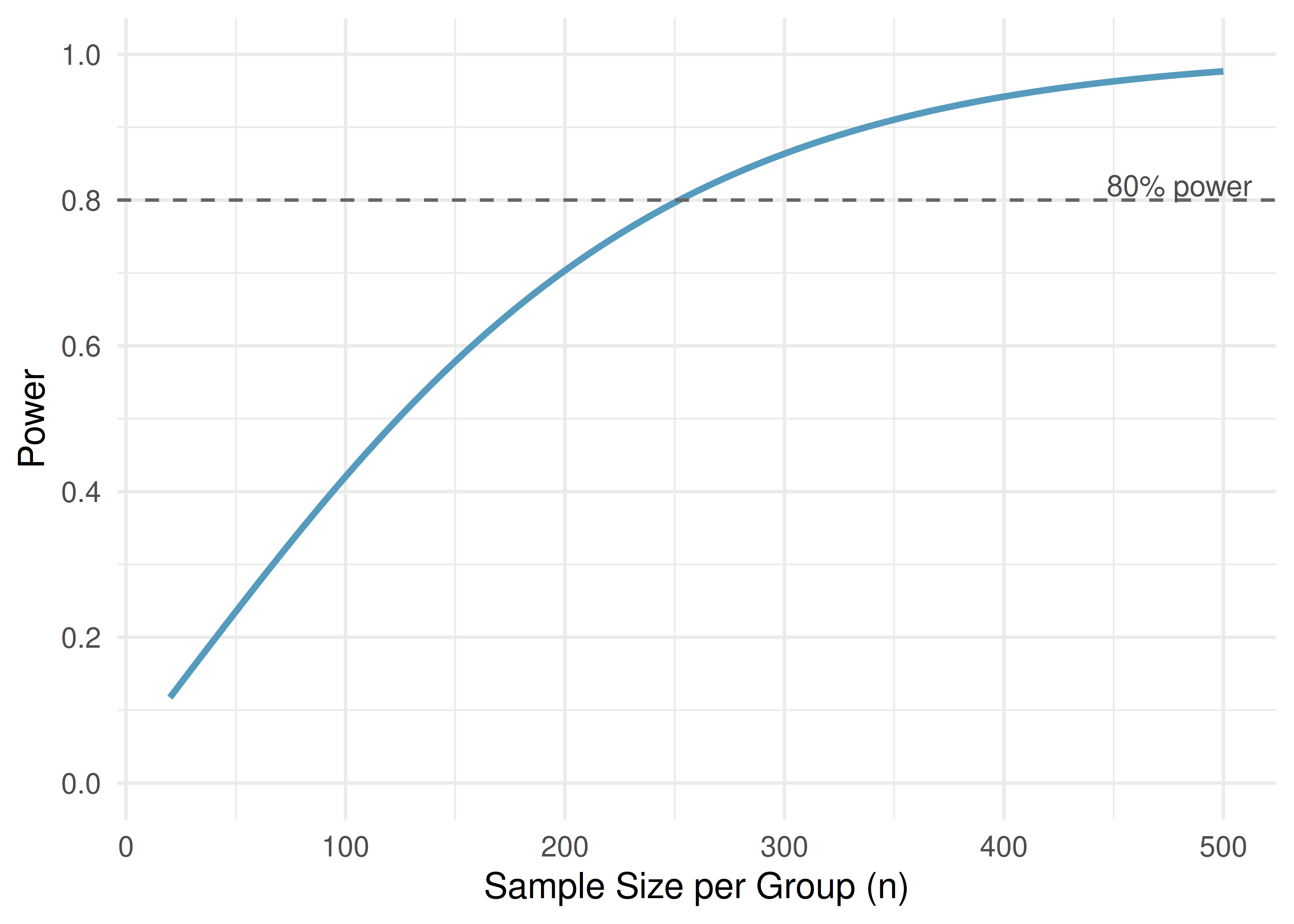
The most common power curve plots power on the y-axis against sample size on the x-axis, for a fixed effect size, \(\alpha\), and \(\sigma\). This curve answers: “How many observations do I need to achieve a desired level of power?”

Figure 30.1: A power curve showing power (y-axis) versus sample size per group (x-axis) for the blood pressure example with true effect = 3 mmHg, σ = 12, α = 0.05. The dashed horizontal line marks 80% power; the curve crosses it at approximately n = 250 per group. ↗ Try this live — drag the \(n\) slider in the Power & Error Visualizer and trace the curve yourself.

Key features of power curves:

• Power starts low for small sample sizes and increases toward 1 as \(n\) grows.
• The curve has a characteristic S-shape: power increases slowly at first, then more rapidly in the middle range, then levels off as it approaches 1.
• The curve never reaches exactly 1 (there is always some chance of a Type II error, though it becomes negligibly small for very large \(n\)).
• The steepest part of the curve — where adding more observations gives the biggest payoff in power — is typically in the middle range.

30.5.2 Power vs. effect size

We can also plot power against effect size, holding \(n\), \(\alpha\), and \(\sigma\) fixed. This curve shows how the detectable effect depends on its magnitude.

Figure 30.2: A power curve showing power (y-axis) versus true effect size (x-axis) for the blood pressure example with n = 200 per group, σ = 12, α = 0.05. Larger effects are easier to detect. ↗ Try this live — drag the effect-size slider and watch power respond.

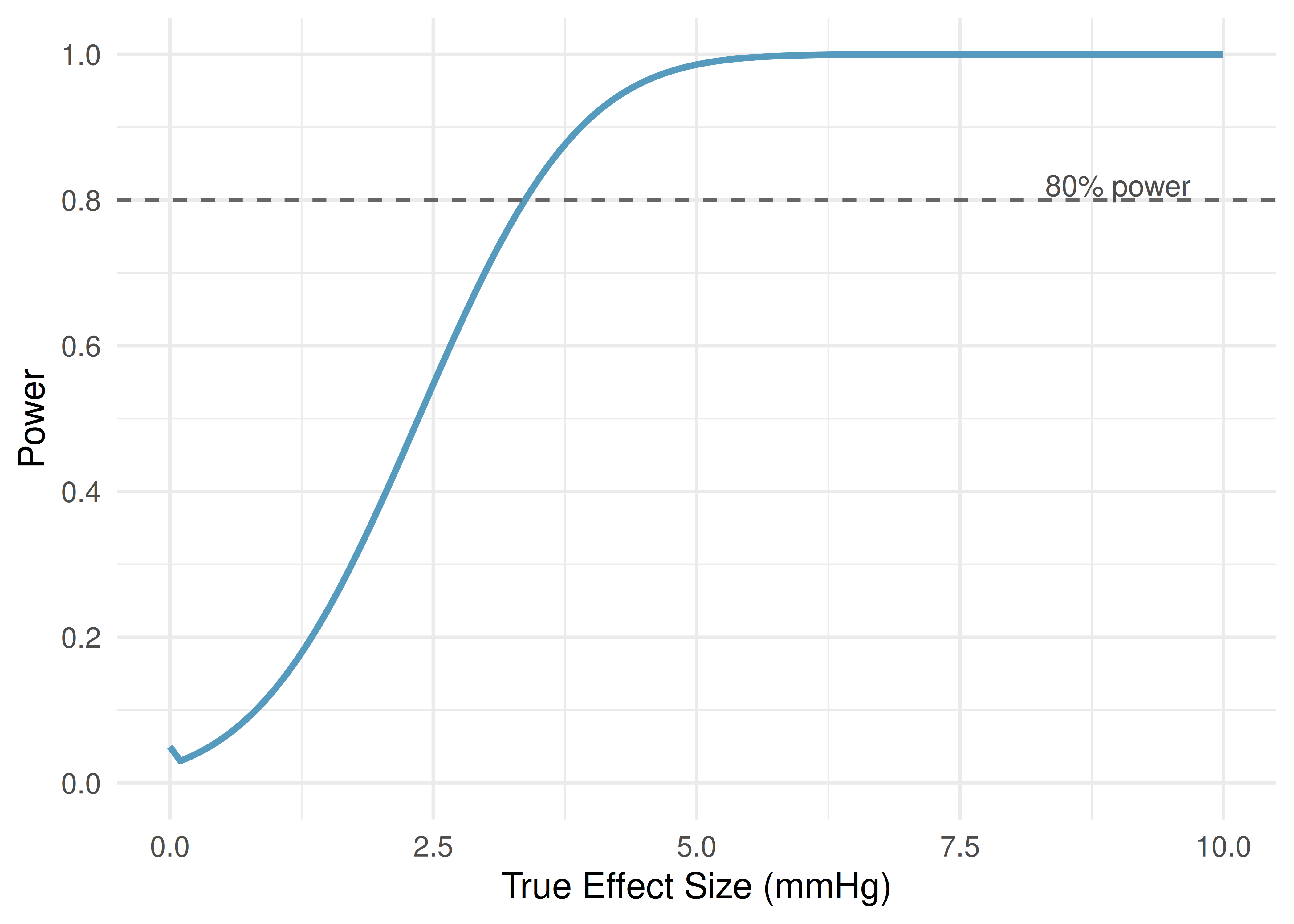
At an effect size of 0, the “power” is just \(\alpha\) — this is the Type I error rate, the probability of rejecting \(H_0\) when there is no effect. As the effect size grows, power increases.

Look at the power-vs-sample-size curve description above. If a researcher can only afford to recruit 100 patients per group, approximately what power would she have? Is this adequate?

Show answer

From the curve, at \(n = 100\) per group the power is approximately 42%. This is far below the conventional minimum of 80%. The researcher should either find a way to increase the sample size, or reconsider whether the study is worth conducting at this scale.

30.6 Typical power targets

How much power is “enough”? There is no universal answer, but strong conventions have emerged in statistical practice.

The 80% power convention. The most widely used target is power = 0.80 (80%). This means the study has an 80% chance of detecting the specified effect. Equivalently, \(\beta = 0.20\) — a 20% chance of a Type II error.

Some fields or funding agencies require higher power:

• 80% power is the conventional minimum for most research.
• 90% power is sometimes required for clinical trials, especially when the consequences of a Type II error are severe.
• 95% power is occasionally used in high-stakes contexts but requires substantially larger sample sizes.

Why is 80% a reasonable target? Why not 95% or 99%?

---

The choice of 80% reflects a practical tradeoff. Increasing power beyond 80% requires increasingly large sample sizes, and the gains become smaller. Going from 80% to 90% power might require 30-50% more observations. Going from 90% to 95% might require another 30% or more. At some point, the cost and logistical difficulty of recruiting additional participants outweigh the marginal reduction in Type II error risk.

The 80% target also reflects the observation that in most settings, a Type II error (missing a real effect) is considered less serious than a Type I error (claiming a false effect), so we are comfortable with \(\beta = 0.20\) even when \(\alpha = 0.05\). If the consequences of missing an effect are severe — for example, in a drug safety trial — a higher power target is appropriate.

Power analysis must be done before data collection. A power analysis conducted after data have been collected and analyzed is called post hoc power analysis (or “observed power”), and it is widely regarded as misleading. Post hoc power is mathematically determined by the p-value and adds no new information. The time to think about power is during the study design phase.

30.7 Computing power for a two-sample test

While a full derivation of power formulas is beyond the scope of this course, it is useful to see the mechanics of a power calculation for the common case of comparing two group means. This section walks through the logic step by step using the blood pressure medication example.

30.7.1 Setting up the null and alternative distributions

Suppose a pharmaceutical company has developed a new drug to lower blood pressure. They plan a randomized experiment comparing the new drug to a standard medication. The hypotheses are:

• \(H_0\): \(\mu_{\text{treatment}} - \mu_{\text{control}} = 0\) (no difference)
• \(H_A\): \(\mu_{\text{treatment}} - \mu_{\text{control}} \neq 0\) (there is a difference)

From pilot studies, the standard deviation of blood pressure measurements within each group is about \(\sigma = 12\) mmHg. The test will use \(\alpha = 0.05\).

Step 1: Determine the null distribution. Under \(H_0\), the difference \(\bar{x}_{\text{treatment}} - \bar{x}_{\text{control}}\) has mean 0 and standard error:

\[SE = \sqrt{\frac{\sigma^2}{n} + \frac{\sigma^2}{n}} = \sigma\sqrt{\frac{2}{n}}\]

With \(n = 100\) per group: \(SE = 12\sqrt{2/100} = 12 \times 0.1414 = 1.70\).

So under \(H_0\), the test statistic approximately follows a normal distribution centered at 0 with standard deviation 1.70.

Step 2: Find the rejection regions. At \(\alpha = 0.05\) (two-sided), we reject \(H_0\) when the observed difference falls more than \(1.96 \times SE = 1.96 \times 1.70 = 3.33\) units from zero. That is, we reject when the observed difference is below \(-3.33\) or above \(+3.33\).

Step 3: Specify the alternative. Suppose the new drug truly lowers blood pressure by 3 mmHg more than the standard medication, so the true difference is \(\mu_{\text{treatment}} - \mu_{\text{control}} = -3\).

Under this alternative, the observed difference follows a normal distribution centered at \(-3\) with standard deviation 1.70 (the standard error doesn’t change — it depends on \(\sigma\) and \(n\), not the true mean).

Step 4: Compute the power. Power is the probability that the observed difference falls in the rejection region when the alternative is true. The rejection boundary closest to the true effect of \(-3\) is at \(-3.33\). So we need:

\[P(\bar{x}_{\text{treatment}} - \bar{x}_{\text{control}} < -3.33 \mid \text{true difference} = -3)\]

Standardizing:

\[Z = \frac{-3.33 - (-3)}{1.70} = \frac{-0.33}{1.70} = -0.20\]

\[P(Z < -0.20) \approx 0.42\]

The power is approximately 42%. This is quite low — the study has less than a coin-flip chance of detecting the 3 mmHg effect.

Using the same setup (\(\sigma = 12\), \(\alpha = 0.05\), true effect \(= -3\) mmHg), compute the power when \(n = 250\) per group.

Show answer

With \(n = 250\): \(SE = 12\sqrt{2/250} = 12 \times 0.0894 = 1.073\). Rejection boundary: \(1.96 \times 1.073 = 2.10\). Under \(H_A\) centered at \(-3\): \(Z = (-2.10 - (-3)) / 1.073 = 0.90/1.073 = 0.84\). \(P(Z < 0.84) \approx 0.80\). The power is approximately 80% — right at the conventional target. So about 250 patients per group would be needed to achieve 80% power for this effect size.

30.8 Chapter review

30.8.1 Summary

Power is the probability of correctly rejecting a false null hypothesis: Power \(= 1 - \beta\). A well-designed study should have power of at least 0.80 (80%), meaning it has an 80% chance of detecting the effect of interest.

Power depends on four factors: sample size (more data gives more power), effect size (larger effects are easier to detect), discernibility level (higher \(\alpha\) gives more power but more false alarms), and population variability (less variability gives more power). Of these, sample size is the factor most under the researcher’s control.

When exact power formulas are unavailable, simulation provides a flexible alternative: generate many datasets under the assumed alternative, run the test on each, and count the proportion that reject \(H_0\). Power curves visualize how power changes with sample size or effect size, helping researchers identify the “sweet spot” where power is adequate without wasting resources.

Power analysis should always be done before data collection. Post hoc power analysis — computing power after the study is over — is misleading and widely discouraged.

30.9 Exercises

StatLens Exercises

Let StatLens do the arithmetic; spend your effort on the reasoning a calculator can’t do.

1. Read power off the dual-curve picture. Open the Power & Error Visualizer.

   1. Identify the two curves on the plot. Which is the null distribution and which is the alternative? How do you tell?
   2. The shaded regions correspond to \(\alpha\), \(\beta\), and power. Match each label to the correct region.
   3. Read off the current power (the tool reports it as a number). At \(\alpha = 0.05\), \(n = 30\), \(\delta = 1\), \(\sigma = 2\), what is it?
   4. In one sentence, explain what “power \(= 0.5\)” would mean in plain English about your experiment.

2. The four levers — vary one at a time. Stay in the Power & Error Visualizer.

   1. Start at \(\alpha = 0.05\), \(n = 30\), \(\delta = 1\), \(\sigma = 2\). Note the power. Now double \(n\) to 60. How does power change?
   2. Reset to defaults. Double \(\delta\) (effect size) to 2. How does power change compared to doubling \(n\)? Which is the bigger lever?
   3. Reset. Double \(\sigma\) (population noise) to 4. What happens to power? Why?
   4. Reset. Lower \(\alpha\) from 0.05 to 0.01. What happens to power? Why is there a tradeoff?

3. Simulation as a sanity check. Open the Power Lab (simulation).

   1. Run 500 simulated \(z\)-tests under these parameters. The empirical reject rate is the simulated power. How close is it to the analytic power from Exercise 1?
   2. Run 5000 simulations and re-read. Tighter agreement?
   3. Look at the dance-of-the-p-values panel. Under a real effect, p-values are not uniform — where do they cluster? Why?
   4. A student says: “If the analytic power formula already gives the answer, the simulation is pointless.” Give two reasons the simulation is still valuable.

4. Reading studies from the power perspective. A journal article reports: “A previous trial (\(n = 80\), \(\alpha = 0.05\)) failed to detect an effect of [the new drug] on blood pressure.” A second team plans a replication with \(n = 200\).

   1. Why does “the previous trial failed to detect” not mean “the drug doesn’t work”?
   2. If the true effect size is small (say \(\delta/\sigma = 0.2\)), use the Power & Error Visualizer to estimate the power of the first trial. Is the failure to detect surprising?
   3. At what \(n\) would the replication achieve at least 80% power for \(\delta/\sigma = 0.2\) and \(\alpha = 0.05\)? Use the tool’s \(n\) slider.
   4. Suppose the replication achieves power 0.85 and the result is still non-significant. What can you conclude — and what can you not?

5. Power, replication, and “statistical significance.” Suppose 100 independent labs run the same experiment with true power 0.8 at \(\alpha = 0.05\).

   1. Roughly how many labs will report a “statistically discernible” result? How many will report a non-result?
   2. Now suppose only the 80 labs with discernible results publish their findings. What kind of bias does this introduce in the literature?
   3. Three independent meta-analyses pool all 100 labs’ results (not just the published ones). What advantage does this have over relying on any single significant study?
   4. A media headline reads: “New study shows X causes Y.” The study was a single trial with power 0.5. Given everything you’ve learned, how should you read this headline?