12 Inference for Proportions

In earlier chapters, we used simulation-based methods to draw conclusions about population proportions. In the randomization tests and bootstrap confidence intervals chapters, we built randomization distributions and bootstrap confidence intervals; in the normal approximation chapter, we learned that the normal distribution provides a mathematical model for these sampling distributions when certain conditions are met. In this chapter, we bring everything together for proportions. We develop normal-based confidence intervals and hypothesis tests for a single proportion and for the difference between two proportions. Throughout, we compare these formula-based results to the simulation-based results from earlier chapters, reinforcing the idea that these are two routes to the same destination.

12.1 Case study: is the complication rate lower?

People providing an organ for donation sometimes seek the help of a special medical consultant. These consultants assist the patient in all aspects of the surgery, with the goal of reducing the possibility of complications during the medical procedure and recovery.

One consultant tried to attract patients by noting the national complication rate for liver donor surgeries is about 10%, but her clients have had only 3 complications in the 62 liver donor surgeries she has facilitated. She claims this is strong evidence that her work reduces complications.

Let $p$ denote the true complication rate for this consultant’s clients. The point estimate is \[\hat{p} = \frac{3}{62} = 0.048.\]

The sample rate 4.8% is well below the national 10%. But we saw the same puzzle in the sampling variability chapter: even when nothing is going on, sample proportions vary from sample to sample. Could a rate as low as 4.8% out of 62 have happened by chance, if the true rate really were 10%? That is the question a hypothesis test is built to answer:

$H_0$: The consultant’s true complication rate matches the national rate, $p = 0.10$.
$H_A$: The consultant’s true complication rate is lower, $p < 0.10$.

To weigh the evidence, we need to know how much $\hat{p}$ would vary from sample to sample if $H_0$ were true. That variability is captured by the null distribution of $\hat{p}$.

12.2 Building the null distribution by simulation

We do not need calculus or a formula to picture the null distribution — we can build it directly with simulation. This mirrors the logic of the randomization tests chapter, applied here to a single proportion.

12.2.1 The marbles metaphor

Imagine a large bag of marbles: 10% orange (complication) and 90% blue (no complication). This bag models the world under $H_0$. Each surgery is one draw from the bag; a “study” of $n = 62$ surgeries is one scoop of 62 marbles. The proportion of orange marbles in the scoop is one simulated $\hat{p}_{sim}$ from the null distribution.

If we scoop 62 marbles and get 5 orange and 57 blue, then \[\hat{p}_{sim1} = \frac{5}{62} = 0.081.\]

That is one simulated study. Under $H_0$, this could easily have happened, even though it does not equal 0.10 exactly.

Is one simulated $\hat{p}_{sim}$ enough to draw a conclusion about the consultant?

No. One draw tells us nothing about the shape of the null distribution — it is a single value that happens to land somewhere by chance. To know what values of $\hat{p}$ are typical and which are extreme under $H_0$, we need many simulations.

12.2.2 From one draw to many

The natural next question is: what happens as we accumulate more draws? Does the null distribution take a recognizable shape? Does it settle down or keep drifting?

This is the moment where a static picture struggles. Jumping from “one draw at $\hat{p}_{sim1} = 0.081$” to a smooth histogram of 10,000 draws is a big cognitive leap when you have not seen this before. It is worth pausing to build the distribution one increment at a time.

Predict → Do → Explain. Open the Sampling Distribution Lab (proportion mode) — preloaded with $p = 0.10$ and $n = 62$, the null-hypothesis world for the medical-consultant case. The gated activity opens with a Predict step (commit to where the distribution of $\hat{p}_{sim}$ will be centered, how spread out, and what shape), walks you through drawing 1, 10, 100, and 1,000 samples in sequence, and closes with an Explain step where you articulate what the buildup showed. Your responses save locally in the tool, so you can return to your work on the same device.

Three ideas the activity lands on — worth flagging in the reading so you can compare them to your own conclusions:

More samples do not make the individual $\hat{p}_{sim}$ values more precise — they fill in the same null distribution. To get narrower $\hat{p}_{sim}$ values you must increase $n$ (the size of each scoop), not the number of scoops.
The null distribution has a stable center at $p = 0.10$ and a stable spread even while the individual draws stay noisy. That stability is what makes the p-value calculation possible.
The distribution is roughly bell-shaped, but with a mild right skew. That skew is not noise — it is a signal. With $p = 0.10$ and $n = 62$, the expected number of successes is $np = 6.2 < 10$, so the success–failure condition fails and the normal approximation is only approximate. When $p$ sits near 0 (or 1) and $n$ is not large, $\hat{p}$ has more room to wander toward the middle than toward the floor, which pushes a tail out to the right. This is the case where a simulated null distribution is more trustworthy than a normal formula — exactly the situation we started the chapter with.

12.2.3 The null distribution at 1,000 simulations

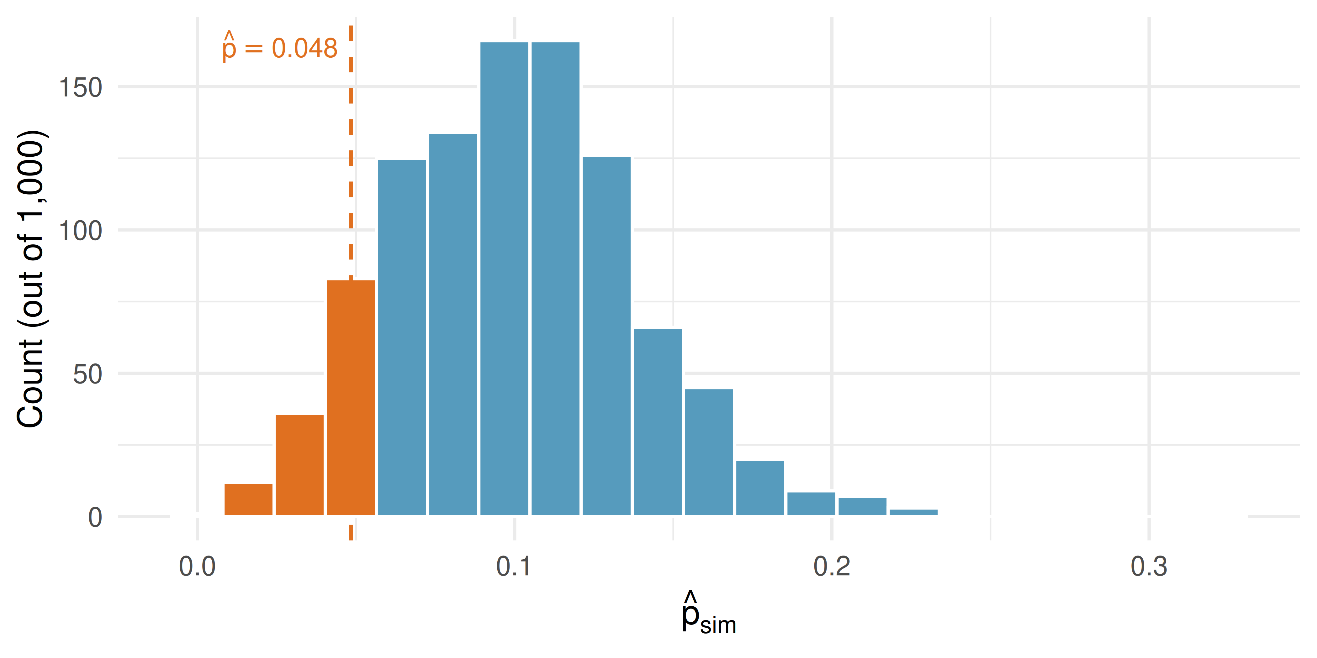
A computer can repeat the marbles scoop as many times as we want. Here are the results of 1,000 simulated studies under $H_0$: each study draws 62 marbles from the 10% / 90% bag, and we record $\hat{p}_{sim}$ from each.

Histogram of 1,000 simulated sample proportions under a null proportion of 0.10 with sample size 62. The distribution is centered near 0.10 and roughly bell-shaped but slightly right-skewed. The left tail at or below 0.048 is shaded. — Figure 12.1: The null distribution of p-hat from 1,000 simulated studies under H₀: p = 0.10, n = 62. Simulations with p-hat ≤ 0.048 (as extreme as the consultant’s observed value, or more extreme) are shaded orange. ↗ Try this live — simulate under $H_0$ with your own $p$ and $n$ and rebuild the null.

Two observations to record before we compute anything:

The distribution is centered near $p = 0.10$. That is not luck — it is because we built it under $H_0$, where the truth is $p = 0.10$. Simulated $\hat{p}$ values scatter symmetrically-ish around that center.
The distribution has a shape we can measure. It looks roughly bell-shaped but with a mild right skew, because $p = 0.10$ is close to 0 and $\hat{p}$ cannot go below zero.

12.2.4 Reading the p-value

The consultant’s observed $\hat{p} = 0.048$ is marked with the dashed line. The orange-shaded bars are the simulated $\hat{p}_{sim}$ values that are at least as extreme as the observed value in the direction of the alternative — here, $\hat{p}_{sim} \leq 0.048$.

The p-value is the fraction of the simulated studies that landed in the shaded tail:

\[\text{p-value} \;=\; \frac{\text{simulations with } \hat{p}_{sim} \leq 0.048}{1{,}000} \;\approx\; 0.132.\]

Using $\alpha = 0.05$, what conclusion should we draw?

The p-value $\approx 0.132$ is greater than $\alpha = 0.05$. We fail to reject $H_0$. The data do not provide convincing evidence that the consultant’s true complication rate is lower than the national 10% — a rate of 3 in 62 could plausibly occur even if her true rate were 10%.

Failing to reject $H_0$ is not the same as concluding that her rate equals 10%. It only says the data are compatible with the national rate; a larger study would be needed to distinguish a small real improvement from chance.

Simulating the null distribution of $\hat{p}$.

Whenever we want to test $H_0: p = p_0$ but a normal-based formula is unreliable, we can build the null distribution directly:

Set up a marbles-bag with the proportion $p_0$ specified by $H_0$.
Repeatedly scoop $n$ marbles and record the simulated $\hat{p}_{sim}$.
Read the p-value as the tail area of the null distribution beyond the observed $\hat{p}$.

This works for any sample size and does not require the success–failure condition. The formula-based approach in the next section is faster when its conditions are met, but the simulation is always available as a backup.

12.3 Normal approximation for proportions

12.3.1 The sampling distribution of $\hat{p}$

In the normal approximation chapter, we saw that the Central Limit Theorem guarantees that the sampling distribution of $\hat{p}$ is approximately normal when certain conditions are met. Let’s state these conditions precisely.

Sampling distribution of $\hat{p}$.

The sampling distribution of the sample proportion $\hat{p}$, based on a sample of size $n$ from a population with true proportion $p$, is approximately normal when:

Independence. The observations are independent (e.g., from a simple random sample).
Success-failure condition. We expect to see at least 10 successes and 10 failures: $np \geq 10$ and $n(1-p) \geq 10$.

When these conditions are met, the sampling distribution is approximately:

\[\hat{p} \sim N\!\left(p,\ \sqrt{\frac{p(1-p)}{n}}\right)\]

The success-failure condition requires that the expected number of successes ($np$) and the expected number of failures ($n(1-p)$) are both at least 10. This ensures the sampling distribution of $\hat{p}$ is not too skewed for the normal approximation to work well.

A medical consultant facilitated 62 liver transplant surgeries, with 3 complications. Under the null hypothesis that the true complication rate is $p_0 = 0.10$, is it appropriate to use the normal approximation?

Check the success-failure condition using $p_0 = 0.10$:

Expected successes (complications): $np_0 = 62 \times 0.10 = 6.2$
Expected failures: $n(1-p_0) = 62 \times 0.90 = 55.8$

The expected number of successes (6.2) is less than 10. The success-failure condition is not met, so the normal approximation should not be used here. A simulation-based approach (such as the parametric bootstrap from the bootstrap confidence intervals chapter) would be more appropriate.

A poll surveys 826 randomly selected payday loan borrowers and finds that 51% support a new regulation. Check whether the normal approximation can be used to model $\hat{p}$ for a hypothesis test with $H_0: p = 0.50$.

Show answer

Check the success-failure condition using $p_0 = 0.50$: $np_0 = 826 \times 0.50 = 413$ and $n(1-p_0) = 826 \times 0.50 = 413$. Both are well above 10, so the success-failure condition is met. Combined with the random sample (independence), the normal approximation is appropriate.

12.3.2 The standard error of $\hat{p}$

Standard error of $\hat{p}$.

When conditions are met, the variability of $\hat{p}$ is described by:

\[SE(\hat{p}) = \sqrt{\frac{p(1-p)}{n}}\]

Since we rarely know the true $p$:

For confidence intervals, use $\hat{p}$ as the best guess: $SE = \sqrt{\frac{\hat{p}(1-\hat{p})}{n}}$
For hypothesis tests, use $p_0$ (the value from $H_0$): $SE = \sqrt{\frac{p_0(1-p_0)}{n}}$

Consider polls of size 300 where approximately 2/3 of voters support legalized marijuana. Calculate the standard error of $\hat{p}$.

Show answer

Using $p \approx 2/3$: $SE = \sqrt{\frac{(2/3)(1/3)}{300}} = \sqrt{\frac{2/9}{300}} = \sqrt{0.000741} = 0.027$.

12.4 Confidence interval for a single proportion

12.4.1 The formula

Confidence interval for a single proportion $p$.

\[\hat{p} \pm z^* \times \sqrt{\frac{\hat{p}(1-\hat{p})}{n}}\]

where $z^*$ is the critical value for the desired confidence level (e.g., $z^* = 1.96$ for 95%).

Steps:

Check conditions: independence and success-failure using $\hat{p}$.
Compute $SE$ using $\hat{p}$.
Apply the confidence interval formula.

12.4.2 Worked example: Payday loan regulation

A simple random sample of 826 payday loan borrowers was surveyed, and 70% supported new regulations on payday lenders. Construct a 95% confidence interval for the true proportion who support the regulations.

Step 1: Check conditions.

Independence. The data are a random sample.
Success-failure condition. Using $\hat{p} = 0.70$: $n\hat{p} = 826 \times 0.70 = 578$ and $n(1-\hat{p}) = 826 \times 0.30 = 248$. Both are well above 10.

Step 2: Compute SE.

\[SE = \sqrt{\frac{0.70 \times 0.30}{826}} = \sqrt{\frac{0.21}{826}} = \sqrt{0.000254} = 0.016\]

Step 3: Construct the interval.

\[0.70 \pm 1.96 \times 0.016 = 0.70 \pm 0.031 = (0.669, 0.731)\]

We are 95% confident that between 66.9% and 73.1% of all payday loan borrowers support the new regulation.

12.4.3 Changing the confidence level

The confidence level is controlled by the choice of $z^*$:

Critical values for common confidence levels.
Confidence level	$z^*$	Interval width
90%	1.645	Narrower
95%	1.960	Moderate
99%	2.576	Wider

Higher confidence requires a wider interval – we must cast a wider net to be more confident we have captured the true parameter.

Using the payday loan data ($\hat{p} = 0.70$, $n = 826$, $SE = 0.016$), construct a 99% confidence interval.

Show answer

Using $z^* = 2.576$: $0.70 \pm 2.576 \times 0.016 = 0.70 \pm 0.041 = (0.659, 0.741)$. The 99% interval is wider than the 95% interval, as expected.

A study on stent surgery found a point estimate of 0.090 (the difference in stroke rates) with $SE = 0.028$. Construct a 90% confidence interval.

Show answer

Using $z^* = 1.645$: $0.090 \pm 1.645 \times 0.028 = 0.090 \pm 0.046 = (0.044, 0.136)$. We are 90% confident that stent implantation increases the 30-day stroke rate by between 4.4% and 13.6%.

General confidence interval formula. If a point estimate follows a normal model with standard error $SE$, then a confidence interval for the population parameter is:

\[\text{point estimate} \pm z^* \times SE\]

where $z^*$ corresponds to the chosen confidence level.

Planning a study: choosing $n$

Before collecting data, researchers often need to decide how large a sample to draw. The width of the CI above is driven by the standard error $\sqrt{\hat{p}(1-\hat{p})/n}$, so hitting a target margin of error is really a question of choosing $n$ large enough. We work through the arithmetic (with worst-case $\hat{p} = 0.5$ and other refinements) in the sample size chapter later in the book.

12.5 Hypothesis test for a single proportion

12.5.1 The Z test for a proportion

The test statistic for a single proportion is a Z.

\[Z = \frac{\hat{p} - p_0}{\sqrt{p_0(1 - p_0) / n}}\]

where $\hat{p}$ is the sample proportion and $p_0$ is the hypothesized proportion from $H_0$.

When $H_0$ is true and conditions are met, $Z$ follows a standard normal distribution $N(0, 1)$.

Conditions:

Independent observations
$np_0 \geq 10$ and $n(1 - p_0) \geq 10$

Note that for hypothesis tests, the standard error is computed using $p_0$ (not $\hat{p}$), because we are evaluating the data under the assumption that $H_0$ is true.

12.5.2 Worked example: Support for credit checks

From a random sample of 826 payday loan borrowers, 51% said they would support a regulation requiring lenders to pull credit reports. Is there convincing evidence that a majority (more than 50%) of borrowers support this regulation?

Step 1: State hypotheses.

$H_0$: $p = 0.50$ (no majority support)
$H_A$: $p > 0.50$ (majority support)

This is a one-sided test.

Step 2: Check conditions.

Independence. Random sample.
Success-failure. Using $p_0 = 0.50$: $np_0 = 826 \times 0.50 = 413$ and $n(1-p_0) = 413$. Both $\geq 10$.

Step 3: Compute the test statistic and p-value.

\[SE = \sqrt{\frac{0.50 \times 0.50}{826}} = \sqrt{\frac{0.25}{826}} = 0.017\]

\[Z = \frac{0.51 - 0.50}{0.017} = \frac{0.01}{0.017} = 0.59\]

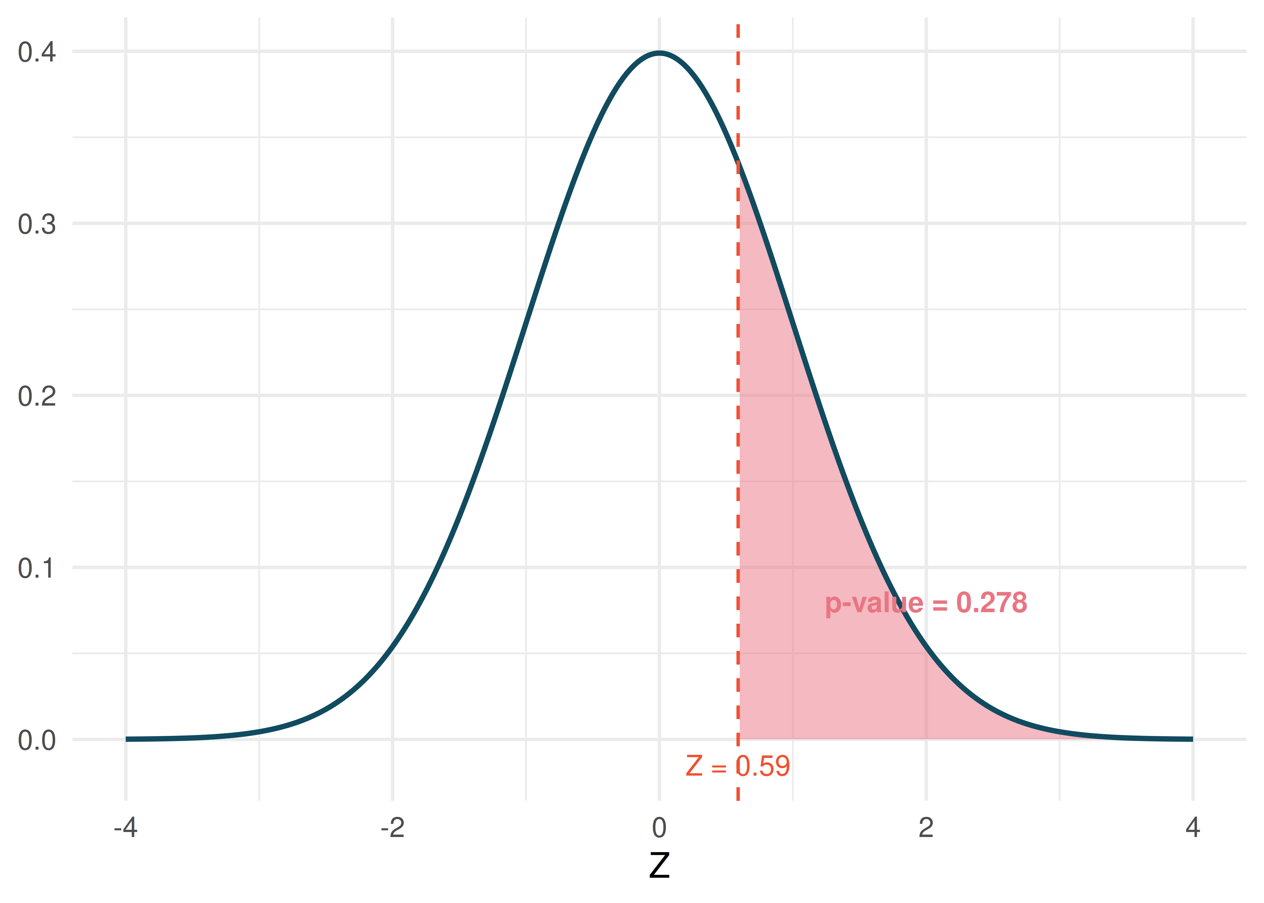
A standard normal distribution curve with the area to the right of Z equals 0.59 shaded. This shaded area represents the p-value for the one-sided test. — Figure 12.2: A standard normal curve with the area to the right of Z = 0.59 shaded, representing the one-sided p-value. ↗ Try this live — drag the cutline to any Z value and read off the right-tail area.

The area to the right of $Z = 0.59$ is 0.278.

Step 4: Conclusion. The p-value of 0.278 is much larger than $\alpha = 0.05$, so we fail to reject $H_0$. The poll does not provide convincing evidence that a majority of payday loan borrowers support the regulation requiring credit checks.

A candidate claims that more than 60% of voters in a district support her. A random sample of 500 voters finds $\hat{p} = 0.64$. Test the claim at $\alpha = 0.05$.

Show answer

Hypotheses: $H_0: p = 0.60$, $H_A: p > 0.60$. Success-failure: $500(0.60) = 300$ and $500(0.40) = 200$, both $\geq 10$. $SE = \sqrt{0.60 \times 0.40 / 500} = \sqrt{0.000480} = 0.0219$. $Z = (0.64 - 0.60)/0.0219 = 1.83$. The right-tail area is 0.034. Since $0.034 < 0.05$, we reject $H_0$. There is sufficient evidence that more than 60% of voters support the candidate.

12.5.3 When conditions fail

When the success-failure condition is not met, the normal model can underestimate the variability of $\hat{p}$, leading to inaccurate p-values and confidence intervals. In these cases, use simulation-based methods:

Bootstrap hypothesis test: Simulate samples under $H_0$ by drawing from a population with proportion $p_0$ (the parametric bootstrap from the bootstrap confidence intervals chapter).
Bootstrap confidence interval: Resample from the original data to estimate the variability of $\hat{p}$.

12.6 Difference of two proportions

12.6.1 The parameter and point estimate

When comparing two groups, the parameter of interest is the difference in population proportions: $p_1 - p_2$. The point estimate is $\hat{p}_1 - \hat{p}_2$.

12.6.2 Confidence interval for a difference in proportions

Confidence interval for $p_1 - p_2$.

\[(\hat{p}_1 - \hat{p}_2) \pm z^* \times \sqrt{\frac{\hat{p}_1(1-\hat{p}_1)}{n_1} + \frac{\hat{p}_2(1-\hat{p}_2)}{n_2}}\]

Conditions:

Independence (extended). Observations are independent within and between groups.
Success-failure condition (each group separately). $n_1\hat{p}_1 \geq 10$, $n_1(1-\hat{p}_1) \geq 10$, $n_2\hat{p}_2 \geq 10$, and $n_2(1-\hat{p}_2) \geq 10$.

In a CPR study, patients who had a heart attack were randomly assigned to receive a blood thinner (treatment) or not (control). The survival rates after 24 hours:

CPR study results.
Group	$n$	Survived	$\hat{p}$
Treatment	50	14	0.280
Control	40	11	0.275

Construct a 90% confidence interval for the difference in survival rates, $p_T - p_C$.

Check conditions.

Independence. Patients were randomly assigned, so groups are independent.
Success-failure. Treatment: $50(0.28) = 14 \geq 10$ and $50(0.72) = 36 \geq 10$. Control: $40(0.275) = 11 \geq 10$ and $40(0.725) = 29 \geq 10$. All conditions met.

Compute the interval.

\[\hat{p}_T - \hat{p}_C = 0.280 - 0.275 = 0.005\]

\[SE = \sqrt{\frac{0.280(0.720)}{50} + \frac{0.275(0.725)}{40}} = \sqrt{\frac{0.2016}{50} + \frac{0.1994}{40}} = \sqrt{0.004032 + 0.004985} = \sqrt{0.009017} = 0.095\]

Using $z^* = 1.645$ for 90% confidence:

\[0.005 \pm 1.645 \times 0.095 = 0.005 \pm 0.156 = (-0.151, 0.161)\]

We are 90% confident that the difference in 24-hour survival rates is between $-15.1\%$ and $+16.1\%$. Because the interval contains 0, we cannot conclude that the blood thinner affects survival rates.

12.6.3 Hypothesis test for a difference in proportions

The test statistic for comparing two proportions is a Z.

\[Z = \frac{(\hat{p}_1 - \hat{p}_2) - 0}{\sqrt{\hat{p}_{pool}(1 - \hat{p}_{pool})\left(\frac{1}{n_1} + \frac{1}{n_2}\right)}}\]

where the pooled proportion is:

\[\hat{p}_{pool} = \frac{\text{total successes in both groups}}{\text{total sample size}} = \frac{x_1 + x_2}{n_1 + n_2}\]

When $H_0$ is true ($p_1 = p_2$), both groups share the same population proportion, so we pool the data to get a single best estimate.

Conditions:

Independence within and between groups.
$n_1\hat{p}_{pool} \geq 10$, $n_1(1-\hat{p}_{pool}) \geq 10$, $n_2\hat{p}_{pool} \geq 10$, $n_2(1-\hat{p}_{pool}) \geq 10$.

Does the blood thinner improve 24-hour survival after CPR? Using the data from the previous example (treatment: 14/50 survived; control: 11/40 survived), test at $\alpha = 0.05$.

Step 1: State hypotheses.

$H_0$: $p_T - p_C = 0$ (the blood thinner has no effect)
$H_A$: $p_T - p_C \neq 0$ (the blood thinner has some effect)

Step 2: Check conditions.

The pooled proportion is $\hat{p}_{pool} = \frac{14 + 11}{50 + 40} = \frac{25}{90} = 0.278$. Check:

$50(0.278) = 13.9 \geq 10$, $50(0.722) = 36.1 \geq 10$
$40(0.278) = 11.1 \geq 10$, $40(0.722) = 28.9 \geq 10$

Conditions are met.

Step 3: Compute the test statistic and p-value.

\[SE = \sqrt{0.278(0.722)\left(\frac{1}{50} + \frac{1}{40}\right)} = \sqrt{0.2007 \times 0.045} = \sqrt{0.009032} = 0.095\]

\[Z = \frac{0.005 - 0}{0.095} = 0.05\]

The two-sided p-value for $Z = 0.05$ is $2 \times P(Z > 0.05) = 2 \times 0.480 = 0.960$.

Step 4: Conclusion. The p-value of 0.960 is far larger than 0.05. We fail to reject $H_0$. There is no evidence that the blood thinner affects 24-hour survival rates.

12.6.4 Why pool for hypothesis tests but not for confidence intervals?

You may have noticed a subtle difference:

Hypothesis tests use the pooled proportion $\hat{p}_{pool}$ in the standard error. This is because under $H_0$, we assume $p_1 = p_2$, so the best estimate of this common proportion comes from combining both samples.
Confidence intervals use the individual sample proportions $\hat{p}_1$ and $\hat{p}_2$ separately. We are not assuming the proportions are equal – we are estimating how different they are.

This distinction applies only to proportions. When we turn to means in the next chapters, we will instead use separate sample standard deviations in both tests and confidence intervals.

12.7 Comparing simulation-based and normal-based methods

Throughout this course, we have developed two parallel approaches to inference:

Comparison of simulation-based and normal approximation approaches.
Feature	Simulation-based	Normal approximation
Requires conditions?	Minimal (mainly independence)	Independence + success-failure
Small samples?	Works well	May be inaccurate
Computational cost	Higher (needs many simulations)	Lower (one formula)
Conceptual clarity	High (directly simulates the process)	Moderate (requires distribution theory)
Precision	Approximate (varies by number of simulations)	Approximate (varies by how well conditions hold)

12.7.1 An example comparison

Consider the opportunity cost study from the randomization tests chapter. The observed difference in proportions was 0.20 ($\hat{p}_T - \hat{p}_C$), and we wanted to test $H_0: p_T - p_C = 0$.

Randomization test (the randomization tests chapter): We shuffled the group labels 10,000 times. The p-value was approximately 0.006.

Normal approximation (this chapter): Using $SE = 0.078$ and $Z = 0.20 / 0.078 = 2.56$, the p-value was 0.005.

Both methods give essentially the same answer and the same conclusion. This is reassuring and typical when conditions are met.

12.7.2 When do they disagree?

The methods can give different answers when:

The success-failure condition fails. The normal approximation may undercount the probability in the tails, leading to p-values that are too small. The simulation approach remains valid.
The sampling distribution is noticeably skewed. The normal model is symmetric by definition, while the true sampling distribution of $\hat{p}$ near 0 or 1 is skewed.

The medical consultant example illustrates this: with only 6.2 expected complications, the normal model gave a p-value of 0.085, while the simulation gave 0.122 – nearly 45% higher. The simulation-based p-value is more trustworthy in this case.

12.7.3 Practical recommendation

When conditions are met: Both methods work. Use the normal approximation for its simplicity, or use simulation for its conceptual directness.
When conditions are borderline or not met: Use simulation. The bootstrap and randomization approaches make fewer assumptions and are more reliable in these settings.
Always check conditions first. The success-failure condition is a simple, quick check that helps you decide which approach to use.

12.8 Explore with StatLens

The Sampling Distribution Lab (proportion mode) builds the sampling distribution of $\hat{p}$ one sample at a time. Set $p = 0.60$ and $n = 50$, watch the distribution fill in, then drop $p$ to $0.05$ to see what happens when the success–failure condition fails.

Analytical tools:

One-Proportion $z$ test + CI, Two-Proportion $z$ test + CI.

Simulation counterparts (for when conditions fail):

12.9 Chapter review

12.9.1 Summary

This chapter developed normal-based inference methods for proportions:

Success-failure condition. The normal approximation for $\hat{p}$ requires at least 10 expected successes and 10 expected failures. For confidence intervals, check with $\hat{p}$; for hypothesis tests, check with $p_0$.
CI for one proportion: $\hat{p} \pm z^* \times \sqrt{\hat{p}(1-\hat{p})/n}$. Use $\hat{p}$ in the SE.
Hypothesis test for one proportion: $Z = \frac{\hat{p} - p_0}{\sqrt{p_0(1-p_0)/n}}$. Use $p_0$ in the SE.
CI for difference of proportions: $(\hat{p}_1 - \hat{p}_2) \pm z^* \times SE$, where $SE$ uses separate sample proportions.
Hypothesis test for difference of proportions: $Z = \frac{\hat{p}_1 - \hat{p}_2}{SE}$, where $SE$ uses the pooled proportion $\hat{p}_{pool}$.
Confidence level is controlled by $z^*$: higher confidence means wider intervals.
When conditions fail (especially the success-failure condition), use simulation-based methods from the randomization tests and bootstrap confidence intervals chapters instead.
Normal-based and simulation-based methods agree when conditions are met and can give different answers when conditions are violated.

12.9.2 Key terms

Success-failure condition, standard error of $\hat{p}$, Z test for a proportion, pooled proportion, confidence interval for a proportion, confidence interval for a difference of proportions, margin of error, critical value ($z^*$), confidence level.

12.10 Exercises

Answers to odd-numbered exercises are provided in the Exercise Solutions appendix at the back of the book.

Do aliens exist? In May 2021, YouGov asked 4,839 adult Great Britain residents whether they think aliens exist, and if so, if they have or have not visited Earth. You want to evaluate if more than a quarter (25%) of Great Britain adults think aliens don’t exist. In the survey 22% responded “I think they exist, and have visited Earth”, 28% responded “I think they exist, but have not visited Earth”, 29% responded “I don’t think they exist”, and 22% responded “Don’t know”. A friend of yours offers to help you with setting up the hypothesis test and comes up with the following hypotheses. Indicate any errors you see.

$H_0: \hat{p} = 0.29 \quad \quad H_A: \hat{p} > 0.29$

Married at 25. A study suggests that the 25% of 25 year-olds have gotten married. You believe that this is incorrect and decide to collect your own sample for a hypothesis test. From a random sample of 776 25 year-olds, you find that 24% of them are married. A friend of yours offers to help you with setting up the hypothesis test and comes up with the following hypotheses. Indicate any errors you see.

$H_0: \hat{p} = 0.24 \quad \quad H_A: \hat{p} \neq 0.24$

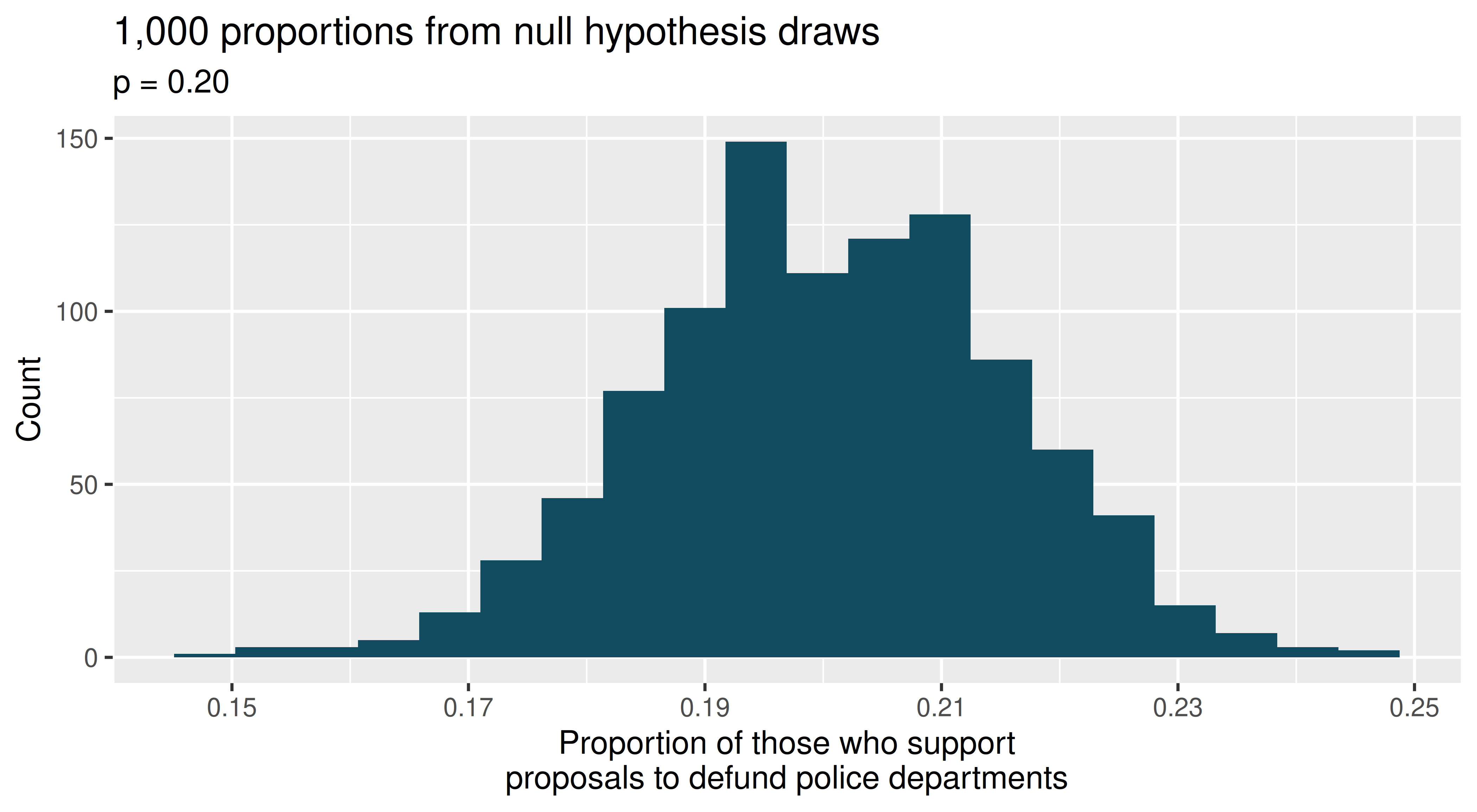
Defund the police. A Survey USA poll conducted in Seattle, WA in May 2021 reports that of the 650 respondents (adults living in this area), 159 support proposals to defund police departments. (Survey USA 2021)

A journalist writing a news story on the poll results wants to use the headline “More than 1 in 5 adults living in Seattle support proposals to defund police departments.” You caution the journalist that they should first conduct a hypothesis test to see if the poll data provide convincing evidence for this claim Write the hypotheses for this test.
Calculate the proportion of Seattle adults in the sample who support proposals to defund police departments.
Describe a setup for a simulation that would be appropriate in this situation and how the p-value can be calculated using the simulation results.
The histogram below shows the distribution of 1,000 $\hat{p}_{sim}$s under the null hypothesis. Estimate the p-value using the plot and use it to evaluate the hypotheses.

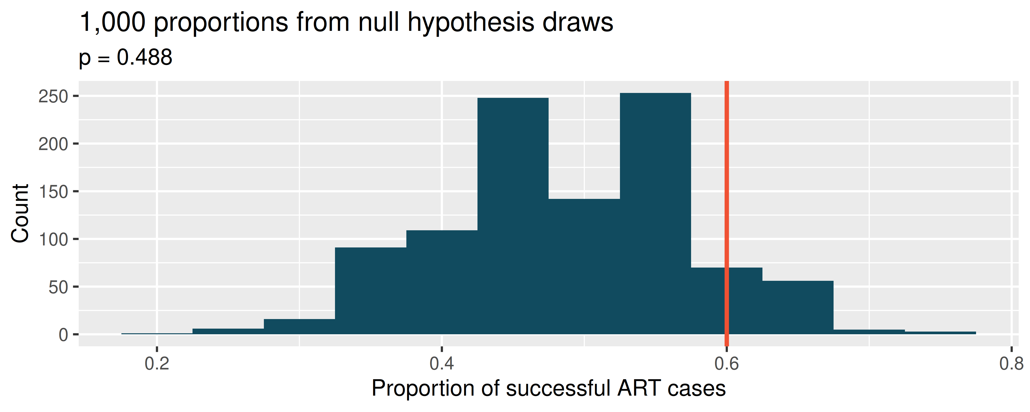
Assisted reproduction. Assisted Reproductive Technology (ART) is a collection of techniques that help facilitate pregnancy (e.g., in vitro fertilization). The 2018 ART Fertility Clinic Success Rates Report published by the Centers for Disease Control and Prevention reports that ART has been successful in leading to a live birth in 48.8% of cases where the patient is under 35 years old. (CDC 2018) A new fertility clinic claims that their success rate is higher than average for this age group. A random sample of 30 of their patients yielded a success rate of 60%. A consumer watchdog group would like to determine if the data provides strong evidence to support the company’s claim.

Write the hypotheses to test if the success rate for ART at this clinic is discernibly higher than the success rate reported by the CDC.
Describe a setup for a simulation that would be appropriate in this situation and how the p-value can be calculated using the simulation results.
The histogram below shows the distribution of 1,000 $\hat{p}_{sim}$s under the null hypothesis. Estimate the p-value using the plot and use it to evaluate the hypotheses.

After performing this analysis, the consumer group releases the following news headline: “Infertility clinic falsely advertises better success rates”. Comment on the appropriateness of this statement.

If I fits, I sits, standard errors. The results of a study on the type of enclosed spaces cats are most likely to sit in show that 5 out of 7 cats chose a square taped to the ground over a shape known as Kanizsa square illusion, which was preferred by the remaining 2 cats. To evaluate whether these data provide convincing evidence that cats prefer one of the shapes over the other, we set $H_0: p = 0.5$, where $p$ is the population proportion of cats who prefer square over the Kanizsa square illusion and $H_A: p \neq 0.5$, which suggests some preference, without specifying which shape is more preferred. (Smith, Chouinard, and Byosiere 2021)

Using the mathematical model, calculate the standard error of the sample proportion in repeated samples of size 7.
A null hypothesis simulation (with 1,000 draws) was run, and the resulting null distribution is displayed in the histogram below. This distribution shows the variability of the sample proportion in samples of size 7 when 50% of cats prefer the square shape over the Kanizsa square illusion. What is the approximate standard error of the sample proportion based on this distribution?

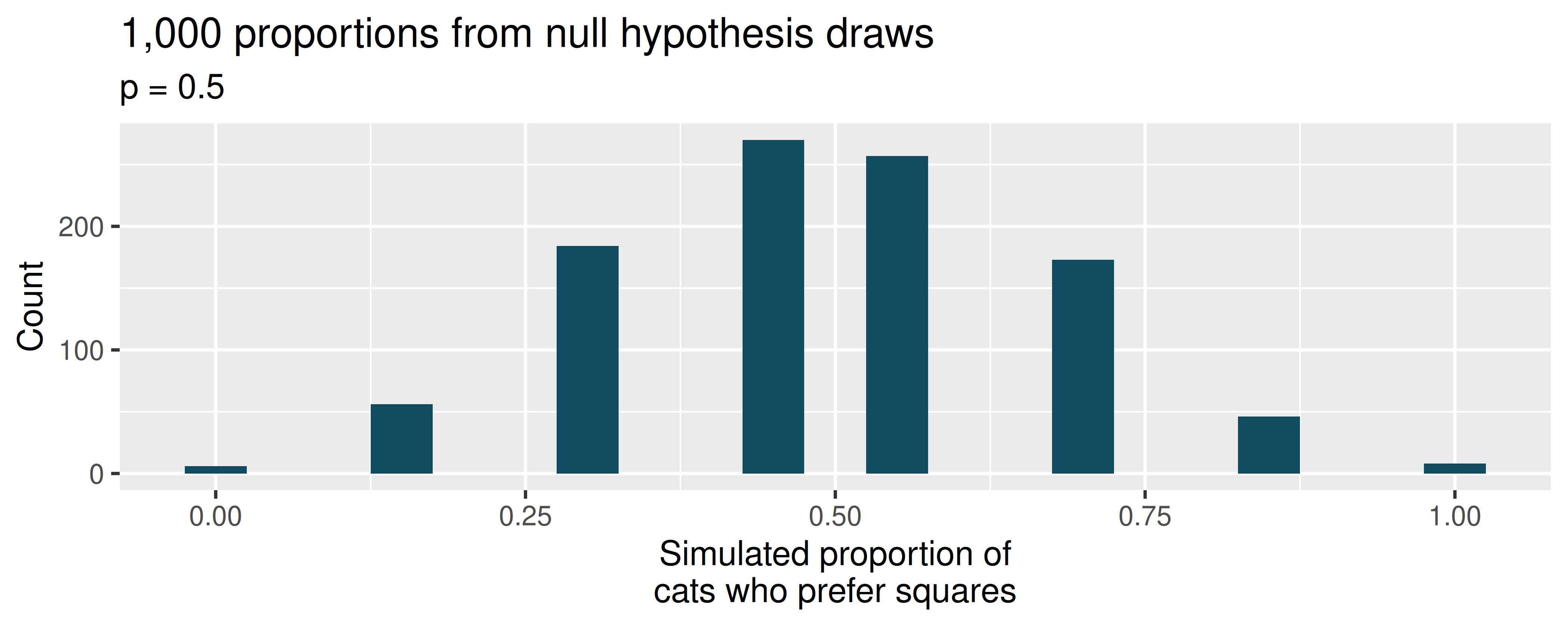
Do the mathematical model and simulated draws yield similar standard errors?
In order to approach the problem using the mathematical model, is the success-failure condition met for this study? Explain.
What features of the null distribution shown above tells us that the mathematical model should probably not be used?

Legalization of marijuana, standard errors. According to the 2022 General Social Survey, in a random sample of 1,207 US adults, 65.3% think marijuana should be made legal. (NORC 2022) Consider a scenario where, in order to become legal, 55% (or more) of voters must approve.

Calculate the standard error of the sample proportion using the mathematical model.
1,000 sample proportions from samples of size 1,207 were drawn from a null distribution where 55% of voters approve legalizing marijuana. The distribution of these proportions is shown in the histogram below. Approximate the standard error of the sample proportion based on this distribution.

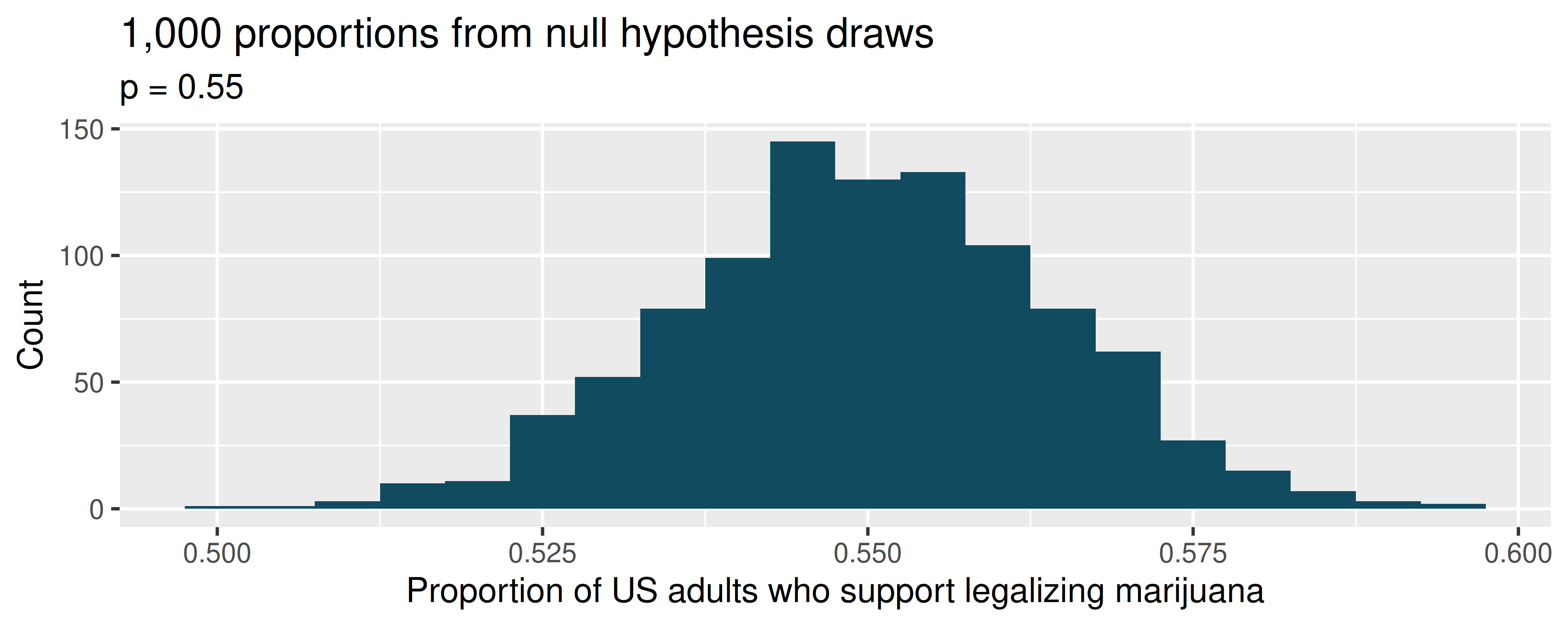
Do the mathematical model and simulated draws yield similar standard errors?
In this setting (to test whether the true underlying population proportion is greater than 0.55), would there be a strong reason to choose the mathematical model over the simulated null hypothesis (or vice versa)?

Statistics and employment, use the bootstrap. In a large university where 70% of the full-time students are employed at least 5 hours per week, the members of the Statistics Department wonder if the same proportion of their students work at least 5 hours per week. They randomly sample 25 majors and find that 15 of the students work 5 or more hours each week.

Two sampling distributions are created to describe the variability in the proportion of statistics majors who work at least 5 hours per week. The null hypothesis distribution imposes a true population proportion of $p=0.7$ while the data bootstrap resamples from the actual data (which has 60% of the observations who work at least 5 hours per week).

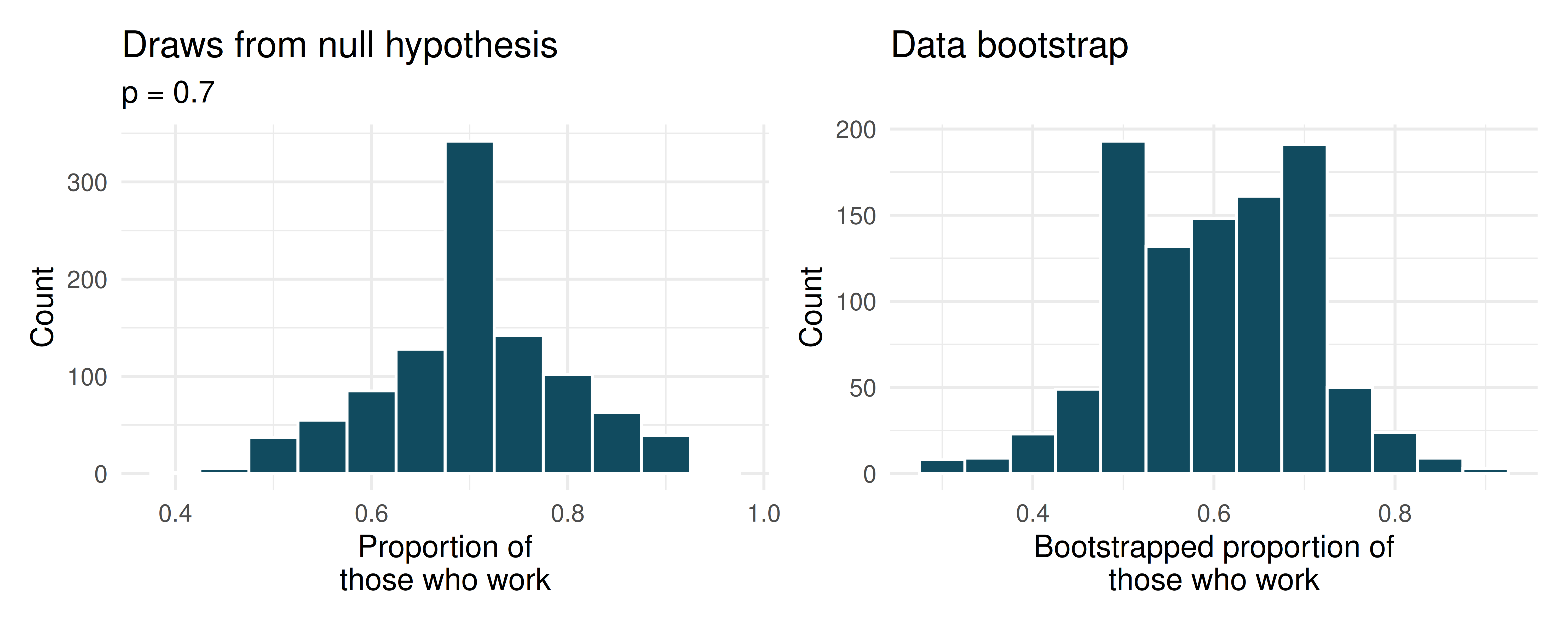
Which distribution should be used to test whether the proportion of all statistics majors who work at least 5 hours per week is 70%? And which distribution should be used to find a confidence interval for the true poportion of statistics majors who work at least 5 hours per week?
Using the appropriate histogram, test the claim that 70% of statistics majors, like their peers, work at least 5 hours per week. State the null and alternative hypotheses, find the p-value, and conclude the test in the context of the problem.
Using the appropriate histogram, find a 98% bootstrap percentile confidence interval for the true proportion of statistics majors who work at least 5 hours per week. Interpret the confidence interval in the context of the problem.
Using the appropriate historgram, find a 98% bootstrap SE confidence interval for the true proportion of statistics majors who work at least 5 hours per week. Interpret the confidence interval in the context of the problem.

CLT for proportions. Define the term “sampling distribution” of the sample proportion, and describe how the shape, center, and spread of the sampling distribution change as the sample size increases when $p = 0.1$.

Vegetarian college students. Suppose that 8% of college students are vegetarians. Determine if the following statements are true or false, and explain your reasoning.

The distribution of the sample proportions of vegetarians in random samples of size 60 is approximately normal since $n \ge 30$.
The distribution of the sample proportions of vegetarian college students in random samples of size 50 is right skewed.
A random sample of 125 college students where 12% are vegetarians would be considered unusual.
A random sample of 250 college students where 12% are vegetarians would be considered unusual.
The standard error would be reduced by one-half if we increased the sample size from 125 to 250.

Young Americans, American dream. About 77% of young adults think they can achieve the American dream. Determine if the following statements are true or false, and explain your reasoning. (Vaughn 2011)

The distribution of sample proportions of young Americans who think they can achieve the American dream in random samples of size 20 is left skewed.
The distribution of sample proportions of young Americans who think they can achieve the American dream in random samples of size 40 is approximately normal since $n \ge 30$.
A random sample of 60 young Americans where 85% think they can achieve the American dream would be considered unusual.
A random sample of 120 young Americans where 85% think they can achieve the American dream would be considered unusual.

Orange tabbies. Suppose that 90% of orange tabby cats are male. Determine if the following statements are true or false, and explain your reasoning.

The distribution of sample proportions of random samples of size 30 is left skewed.
Using a sample size that is 4 times as large will reduce the standard error of the sample proportion by one-half.
The distribution of sample proportions of random samples of size 140 is approximately normal.
The distribution of sample proportions of random samples of size 280 is approximately normal.

Young Americans, starting a family. About 25% of young Americans have delayed starting a family due to the continued economic slump. Determine if the following statements are true or false, and explain your reasoning. (Demos 2011)

The distribution of sample proportions of young Americans who have delayed starting a family due to the continued economic slump in random samples of size 12 is right skewed.
In order for the distribution of sample proportions of young Americans who have delayed starting a family due to the continued economic slump to be approximately normal, we need random samples where the sample size is at least 40.
A random sample of 50 young Americans where 20% have delayed starting a family due to the continued economic slump would be considered unusual.
A random sample of 150 young Americans where 20% have delayed starting a family due to the continued economic slump would be considered unusual.
Tripling the sample size will reduce the standard error of the sample proportion by one-third.

Sex equality. The General Social Survey asked a random sample of 1,390 Americans the following question: “On the whole, do you think it should or should not be the government’s responsibility to promote equality between men and women?” 82% of the respondents said it “should be”. At a 95% confidence level, this sample has 2% margin of error. Based on this information, determine if the following statements are true or false, and explain your reasoning. (NORC 2016)

We are 95% confident that 80% to 84% of Americans in this sample think it’s the government’s responsibility to promote equality between men and women.
We are 95% confident that 80% to 84% of all Americans think it’s the government’s responsibility to promote equality between men and women.
If we considered many random samples of 1,390 Americans, and we calculated 95% confidence intervals for each, 95% of these intervals would include the true population proportion of Americans who think it’s the government’s responsibility to promote equality between men and women.
In order to decrease the margin of error to 1%, we would need to quadruple (multiply by 4) the sample size.
Based on this confidence interval, there is sufficient evidence to conclude that a majority of Americans think it’s the government’s responsibility to promote equality between men and women.

Elderly drivers. A Marist Poll report states that 66% of American adults think licensed drivers should be required to retake their road test once they reach 65 years of age, based on a random sample of 1,018 American adults. They also report a margin of error was 3% at the 95% confidence level. (Poll 2011)

Verify the margin of error reported by The Marist Poll using a mathematical model.
Based on a 95% confidence interval, does the poll provide convincing evidence that more than two thirds of the population think that licensed drivers should be required to retake their road test once they turn 65?

Fireworks on July 4$^{\text{th}}$. A local news outlet reported that 56% of 600 randomly sampled Kansas residents planned to set off fireworks on July $4^{th}$. Determine the margin of error for the 56% point estimate using a 95% confidence level using a mathematical model. (Survey USA 2012)

Proof of COVID-19 vaccination. In the US, businesses and schools shut down due to the COVID-19 pandemic in March 2020, and a vaccine became publicly available for the first time in April 2021. That month, a Gallup poll surveyed a random sample of 3,731 US adults, asking how they felt about the COVID-19 vaccine requirement for air travel. The poll found that 57% said they would favor it. (Gallup 2021b)

Describe the population parameter of interest. What is the value of the point estimate of this parameter?
Check if the conditions required for constructing a confidence interval using a mathematical model based on these data are met.
Construct a 95% confidence interval for the proportion of US adults who favor requiring proof of COVID-19 vaccination for travel by airplane.
Without doing any calculations, describe what would happen to the confidence interval if we decided to use a higher confidence level.
Without doing any calculations, describe what would happen to the confidence interval if we used a larger sample.

Study abroad. A survey on 1,509 high school seniors who took the SAT and who completed an optional web survey shows that 55% of high school seniors are fairly certain that they will participate in a study abroad program in college. (American Council on Education 2008)

Is this sample a representative sample from the population of all high school seniors in the US? Explain your reasoning.
Suppose the conditions for inference are met, regardless of your answer to part (a). Using a mathematical model, construct a 90% confidence interval for the proportion of high school seniors (of those who took the SAT) who are fairly certain they will participate in a study abroad program in college, and interpret this interval in context.
What does “90% confidence” mean?
Based on this interval, would it be appropriate to claim that the majority of high school seniors are fairly certain that they will participate in a study abroad program in college?

Legalization of marijuana, mathematical interval. The General Social Survey asked a random sample of 1,563 US adults: “Do you think the use of marijuana should be made legal, or not?” 60% of the respondents said it should be made legal. (NORC 2022)

Is 60% a sample statistic or a population parameter? Explain.
Using a mathematical model, construct a 95% confidence interval for the proportion of US adults who think marijuana should be made legal, and interpret it in the context of the data.
A critic points out that this 95% confidence interval is only accurate if the statistic follows a normal distribution, or if the normal model is a good approximation. Do the technical conditions hold for these data? Explain.
A news piece on this survey’s findings states, “Majority of US adults think marijuana should be legalized.” Based on your confidence interval, is the news piece’s statement justified?

National Health Plan, mathematical inference. A Kaiser Family Foundation poll for a random sample of US adults in 2019 found that 79% of Democrats, 55% of Independents, and 24% of Republicans supported a generic “National Health Plan”. There were 347 Democrats, 298 Republicans, and 617 Independents surveyed. (Kaiser Family Foundation 2019)

A political pundit on TV claims that a majority of Independents support a National Health Plan. Do these data provide strong evidence to support this type of statement? Your response should use a mathematical model.
Would you expect a confidence interval for the proportion of Independents who oppose the public option plan to include 0.5? Explain.

Is college worth it? Among a simple random sample of 331 American adults who do not have a four-year college degree and are not currently enrolled in school, 48% said they decided not to go to college because they could not afford school. (Pew Research Center 2011)

A newspaper article states that only a minority of the Americans who decide not to go to college do so because they cannot afford it and uses the point estimate from this survey as evidence. Conduct a hypothesis test to determine if these data provide strong evidence supporting this statement.
Would you expect a confidence interval for the proportion of American adults who decide not to go to college because they cannot afford it to include 0.5? Explain.

Taste test. Some people claim that they can tell the difference between a diet soda and a regular soda in the first sip. A researcher wanting to test this claim randomly sampled 80 such people. He then filled 80 plain white cups with soda, half diet and half regular through random assignment, and asked each person to take one sip from their cup and identify the soda as diet or regular. 53 participants correctly identified the soda.

Do these data provide strong evidence that these people are able to detect the difference between diet and regular soda, in other words, are the results discernibly better than just random guessing? Your response should use a mathematical model.
Interpret the p-value in this context.

Will the coronavirus bring the world closer together? In early 2020 the COVID-19 pandemic arrived in the US; by December 2020 the first COVID-19 vaccine was available. An April 2021 YouGov poll asked 4,265 UK adults whether they think the coronavirus bring the world closer together or leave us further apart. 12% of the respondents said it will bring the world closer together. 37% said it would leave us further apart, 39% said it won’t make a difference and the remainder didn’t have an opinion on the matter. (YouGov 2021)

Calculate, using a mathematical model, a 90% confidence interval for the proportion of UK adults who think the coronavirus will bring the world closer together, and interpret the interval in context.
Suppose we wanted the margin of error for the 90% confidence level to be about 0.5%. How large of a sample size would you recommend for the poll?

Quality control. As part of a quality control process for computer chips, an engineer at a factory randomly samples 212 chips during a week of production to test the current rate of chips with severe defects. She finds that 27 of the chips are defective.

What population is under consideration in the dataset?
What parameter is being estimated?
What is the point estimate for the parameter?
What is the name of the statistic that can be used to measure the uncertainty of the point estimate?
Compute the value of the statistic from part (d) using a mathematical model.
The historical rate of defects is 10%. Should the engineer be surprised by the observed rate of defects during the current week?
Suppose the true population value was found to be 10%. If we use this proportion to recompute the value in part (d) using $p = 0.1$ instead of $\hat{p}$, how much does the resulting value of the statistic change?

Nearsighted children. Nearsightedness (myopia) is a common vision condition in which you can see near objects clearly, but farther away objects blurry. It is believed that nearsightedness affects about 8% of all children. In a random sample of 194 children, 21 are nearsighted. Using a mathematical model, conduct a hypothesis test for the following question: do these data provide evidence that the 8% value is inaccurate?

Website registration. A website is trying to increase registration for first-time visitors, exposing 1% of these visitors to a new site design. Of 752 randomly sampled visitors over a month who saw the new design, 64 registered.

Check the conditions for constructing a confidence interval for the proportion of first-time visitors of the site who would register under the new design using a mathematical model.
Compute the standard error which would describe the variability os the point estimate associated with repeated samples of size 752.
Construct and interpret a 90% confidence interval for the fraction of first-time visitors of the site who would register under the new design (assuming stable behaviors by new visitors over time).

Coupons driving visits. A store randomly samples 603 shoppers over the course of a year and finds that 142 of them made their visit because of a coupon they’d received in the mail. Using a mathematical model, construct a 95% confidence interval for the fraction of all shoppers during the year whose visit was because of a coupon they’d received in the mail.

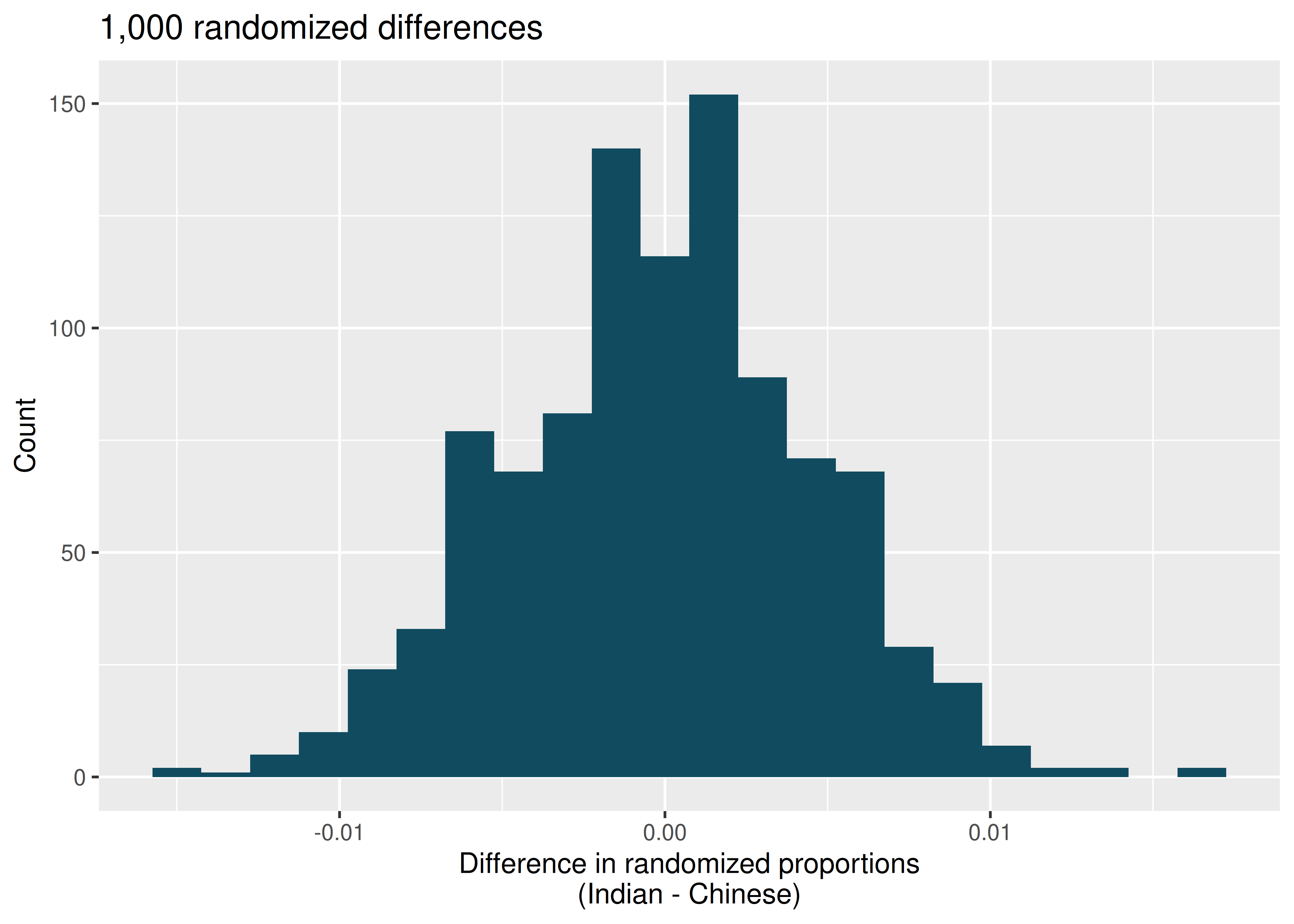
Disaggregating Asian American tobacco use, hypothesis testing. Understanding cultural differences in tobacco use across different demographic groups can lead to improved health care education and treatment. A recent study disaggregated tobacco use across Asian American ethnic groups including Asian-Indian (n = 4,373), Chinese (n = 4,736), and Filipino (n = 4,912), in comparison to non-Hispanic Whites (n = 275,025). The number of current smokers in each group was reported as Asian-Indian (n = 223), Chinese (n = 279), Filipino (n = 609), and non-Hispanic Whites (n = 50,880). (Rao et al. 2021)

To determine whether the proportion of Asian-Indian Americans who are current smokers is different from the proportion of Chinese Americans who are smokers, a randomization simulation was performed.

In both words and symbols provide the parameter and statistic of interest for this study. Do you know the numerical value of either the parameter or statistic of interest? If so, provide the numerical value.
The histogram above provides the sampling distribution (under randomization) for $\hat{p}_{Asian-Indian} - \hat{p}_{Chinese}$ under repeated null randomizations ($\hat{p}$ is the proportion in the sample who are current smokers). Estimate the standard error of $\hat{p}_{Asian-Indian} - \hat{p}_{Chinese}$ based on the randomization histogram.
Consider the hypothesis test to determine if there is a difference in proportion of Asian-Indian Americans as compared to Chinese Americans who are current smokers. Write out the null and alternative hypotheses, estimate a p-value using the randomization histogram, and conclude the test in the context of the problem.

Malaria vaccine effectiveness, hypothesis test. With no currently licensed vaccines to inhibit malaria, good news was welcomed with a recent study reporting long-awaited vaccine success for children in Burkina Faso. With 450 children randomized to either one of two different doses of the malaria vaccine or a control vaccine, 89 of 292 malaria vaccine and 106 out of 147 control vaccine children contracted malaria within 12 months after the treatment. (Datoo et al. 2021)

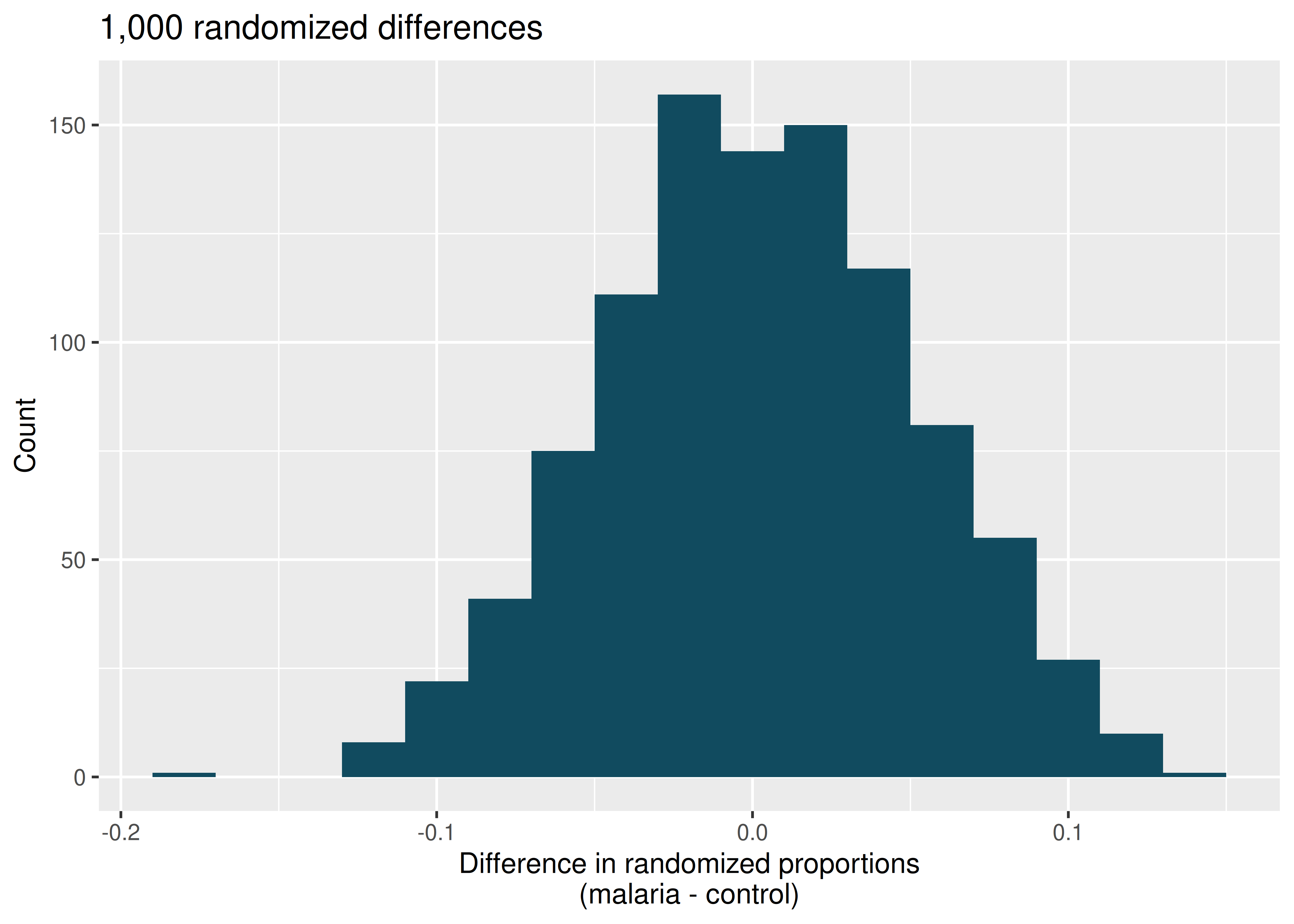
In both words and symbols provide the parameter and statistic of interest for this study. Do you know the numerical value of either the parameter or statisic of interest? If so, provide the numerical value.
The histogram above provides the sampling distribution (under randomization) for $\hat{p}_{malaria} - \hat{p}_{control}$ under repeated null randomizations ($\hat{p}$ is the proportion of children in the sample who contracted malaria). Estimate the standard error of $\hat{p}_{malaria} - \hat{p}_{control}$ based on the randomization histogram.
Consider the hypothesis test constructed to show a lower proportion of children contracting malaria on the malaria vaccine as compared to the control vaccine. Write out the null and alternative hypotheses, estimate a p-value using the randomization histogram, and conclude the test in the context of the problem.

Disaggregating Asian American tobacco use, confidence interval. Based on a study on the degree to which smoking practices differ across ethnic groups. a confidence interval for the difference in current smoking status for Filipino versus Chinese Americans is desired. (Rao et al. 2021)

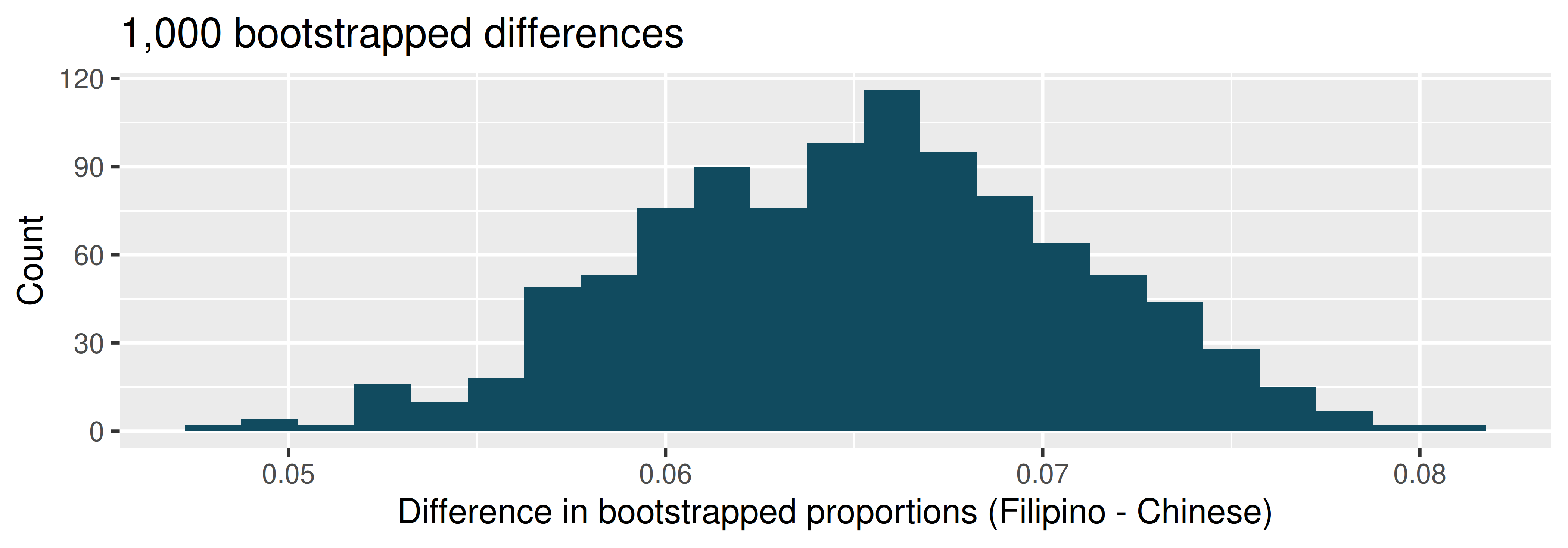
Consider the bootstrap distribution of difference in sample proportions of current smokers (Filipino Americans minus Chinese Americans) in 1,000 bootstrap repetitions as above. Estimate the standard error of the difference in sample proportions, as seen in the histogram.
Using the standard error from the bootstrap distribution, find a 95% bootstrap SE confidence interval for the true difference in proportion of current smokers (Filipino Americans minus Chinese Americans) in the population. Interpret the interval in the context of the problem.
Using the entire bootstrap distribution, find a 95% bootstrap percentile confidence interval for the true difference in proportion of current smokers (Filipino Americans minus Chinese Americans) in the population. Interpret the interval in the context of the problem.

Malaria vaccine effectiveness, confidence interval. With no currently licensed vaccines to inhibit malaria, good news was welcomed with a recent study reporting long-awaited vaccine success for children in Burkina Faso. With 450 children randomized to either one of two different doses of the malaria vaccine or a control vaccine, 89 of 292 malaria vaccine and 106 out of 147 control vaccine children contracted malaria within 12 months after the treatment. (Datoo et al. 2021)

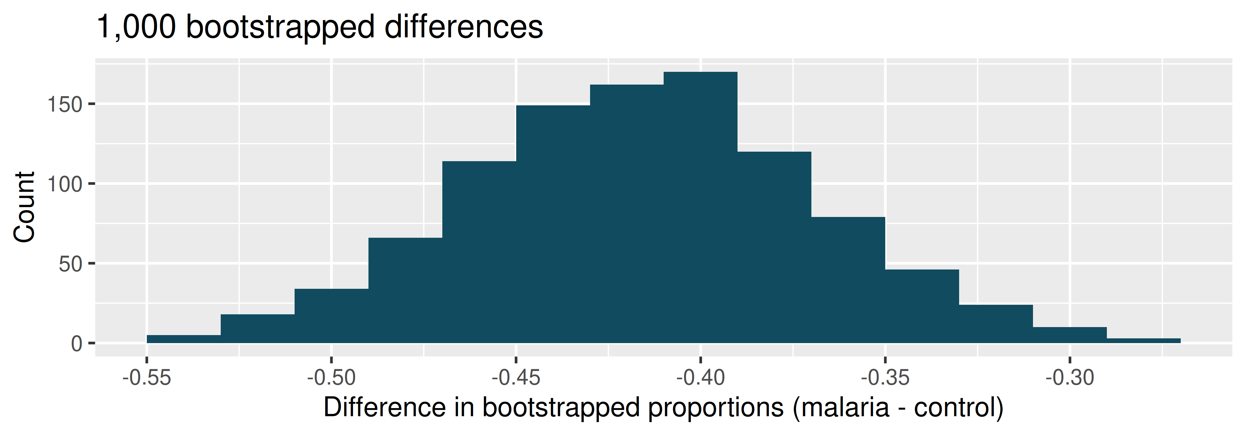
Consider the bootstrap distribution of difference in sample proportions of children who contracted malaria (malaria vaccine minus control vaccine) in 1000 bootstrap repetitions as above. Estimate the standard error of the difference in sample proportions, as seen in the histogram.
Using the standard error from the bootstrap distribution, find a 95% bootstrap SE confidence interval for the true difference in proportion of children who contract malaria (malaria vaccine minus control vaccine) in the population. Interpret the interval in the context of the problem.
Using the entire bootstrap distribution, find a 95% bootstrap percentile confidence interval for the true difference in proportion of children who contract malaria (malaria vaccine minus control vaccine) in the population. Interpret the interval in the context of the problem.

COVID-19 and degree completion. A 2021 Gallup poll surveyed 3,941 students pursuing a bachelor’s degree and 2,064 students pursuing an associate degree (students were not randomly selected but were weighted so as to represent a random selection of currently enrolled US college students). The poll found that 51% of the bachelor’s degree students and 44% of associate degree students said that the COVID-19 pandemic will negatively impact their ability to complete the degree. (Gallup 2021a)

Below are two histograms generated with different computational approaches (both use 1,000 repetitions) to research questions which could be asked of these data. One of the histograms can be used to do a randomization test on whether the proportions of bachelor’s and associate students who think the COVID-19 pandemic will negatively impact their ability to complete the degree. The other histogram is a bootstrap distribution used to quantify the difference in the proportions of bachelor’s and associate’s students who feel this way.

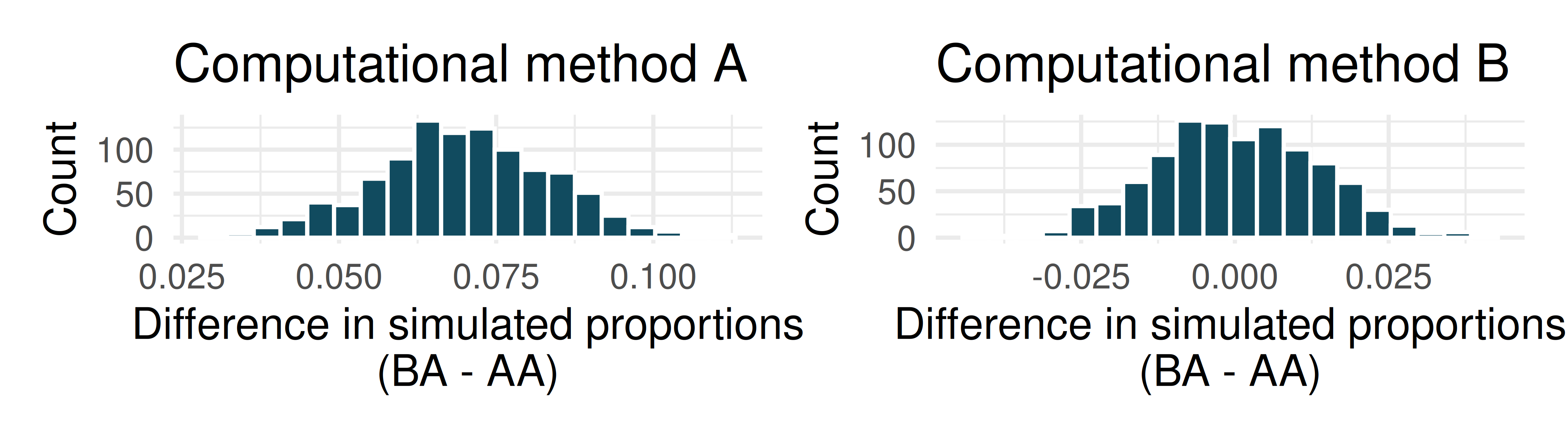
Are the center and standard error of the two graphs approximately the same? Explain.
Write a research question that can be addressed using the histogram generated with computational method A.
Write a research question that can addressed using the histogram generated with computational method B.

Renewable energy. A 2021 Gallup poll surveyed 5,447 randomly sampled US adults who are Republican (or Republican leaning) and 7,962 who are Democrats (or Democrat leaning). 31% of Republicans and 81% of Democrats said “government regulations are necessary to encourage businesses and consumers to rely more on renewable energy sources”. (Gallup 2021a)

Below are two histograms generated with different computational approaches (both use 1,000 repetitions) to research questions which could be asked of these data. One of the histograms can be used to do a randomization test on whether the proportions of Republicans and Democrats who think government regulations are necessary to encourage businesses and consumers to rely more on renewable energy sources are different. The other histogram is a bootstrap distribution used to quantify the difference in the proportions of Republicans and Democrats who agree with this statement.

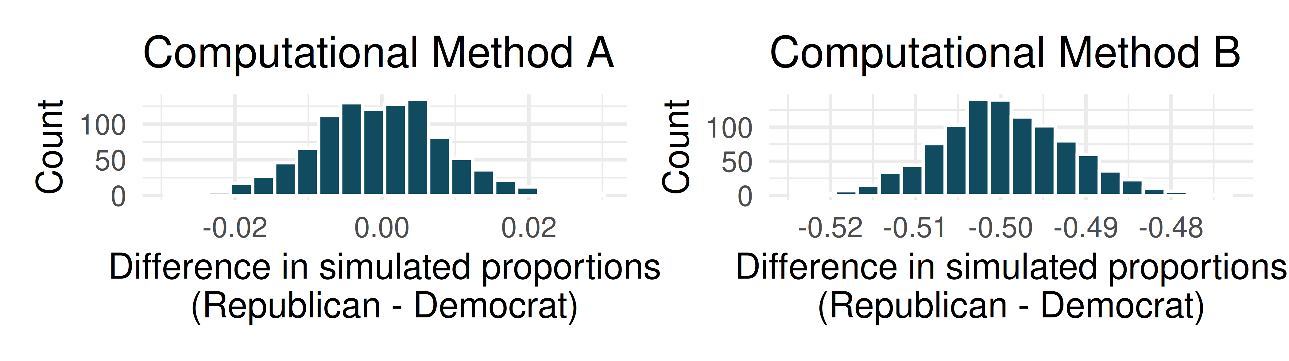
Are the center and standard error of the two graphs approximately the same? Explain.
Write a research question that can addressed using the histogram generated with computational method A.
Write a research question that can addressed using the histogram generated with computational method B.

HIV in sub-Saharan Africa. In July 2008 the US National Institutes of Health announced that it was stopping a clinical study early because of unexpected results. The study population consisted of HIV-infected women in sub-Saharan Africa who had been given single dose Nevaripine (a treatment for HIV) while giving birth, to prevent transmission of HIV to the infant. The study was a randomized comparison of continued treatment of a woman (after successful childbirth) with Nevaripine vs Lopinavir, a second drug used to treat HIV. 240 women participated in the study; 120 were randomized to each of the two treatments. Twenty-four weeks after starting the study treatment, each woman was tested to determine if the HIV infection was becoming worse (an outcome called virologic failure). Twenty-six of the 120 women treated with Nevaripine experienced virologic failure, while 10 of the 120 women treated with the other drug experienced virologic failure. (Lockman et al. 2007)

Create a two-way table presenting the results of this study.
State appropriate hypotheses to test for difference in virologic failure rates between treatment groups.
Complete the hypothesis test and state an appropriate conclusion. (Reminder: Verify any necessary conditions for the test.)

Supercommuters. The fraction of workers who are considered “supercommuters”, because they commute more than 90 minutes to get to work, varies by state. Suppose the 1% of Nebraska residents and 6% of New York residents are supercommuters. Now suppose that we plan a study to survey 1000 people from each state, and we will compute the sample proportions $\hat{p}_{NE}$ for Nebraska and $\hat{p}_{NY}$ for New York.

What is the associated mean and standard deviation of $\hat{p}_{NE}$ in repeated samples of size 1000?
What is the associated mean and standard deviation of $\hat{p}_{NY}$ in repeated samples of size 1000?
Calculate and interpret the mean and standard deviation associated with the difference in sample proportions for the two groups, $\hat{p}_{NY} - \hat{p}_{NE}$ in repeated samples of 1000 in each group.
How are the standard deviations from parts (a), (b), and (c) related?

National Health Plan. A Kaiser Family Foundation poll for US adults in 2019 found that 79% of Democrats, 55% of Independents, and 24% of Republicans supported a generic “National Health Plan”. There were 347 Democrats, 298 Republicans, and 617 Independents surveyed. 79% of 347 Democrats and 55% of 617 Independents support a National Health Plan. (Kaiser Family Foundation 2019)

Calculate a 95% confidence interval for the difference between the proportion of Democrats and Independents who support a National Health Plan $(p_{D} - p_{I})$, and interpret it in this context. We have already checked conditions for you.
True or false: If we had picked a random Democrat and a random Independent at the time of this poll, it is more likely that the Democrat would support the National Health Plan than the Independent.

Sleep deprivation, CA vs. OR, confidence interval. According to a report on sleep deprivation by the Centers for Disease Control and Prevention, the proportion of California residents who reported insufficient rest or sleep during each of the preceding 30 days is 8.0%, while this proportion is 8.8% for Oregon residents. These data are based on simple random samples of 11,545 California and 4,691 Oregon residents. Calculate a 95% confidence interval for the difference between the proportions of Californians and Oregonians who are sleep deprived and interpret it in context of the data. (CDC 2008)

Gender pay gap in medicine. A study examined the average pay for men and women entering the workforce as doctors for 21 different positions. (Lo Sasso et al. 2011)

If each gender was equally paid, then we would expect about half of those positions to have men paid more than women and women would be paid more than men in the other half of positions. Write appropriate hypotheses to test this scenario.
Men were, on average, paid more in 19 of those 21 positions. Complete a hypothesis test using your hypotheses from part (a).

Sleep deprivation, CA vs. OR, hypothesis test. A CDC report on sleep deprivation rates shows that the proportion of California residents who reported insufficient rest or sleep during each of the preceding 30 days is 8.0%, while this proportion is 8.8% for Oregon residents. These data are based on simple random samples of 11,545 California and 4,691 Oregon residents.

Conduct a hypothesis test to determine if these data provide strong evidence that the rate of sleep deprivation is different for the two states. (Reminder: Check conditions)
It is possible the conclusion of the test in part (a) is incorrect. If this is the case, what type of error was made?

Is yawning contagious? An experiment conducted by the MythBusters, a science entertainment TV program on the Discovery Channel, tested if a person can be subconsciously influenced into yawning if another person near them yawns. 50 people were randomly assigned to two groups: 34 to a group where a person near them yawned (treatment) and 16 to a group where there wasn’t a person yawning near them (control). The visualization below displays how many participants yawned in each group.

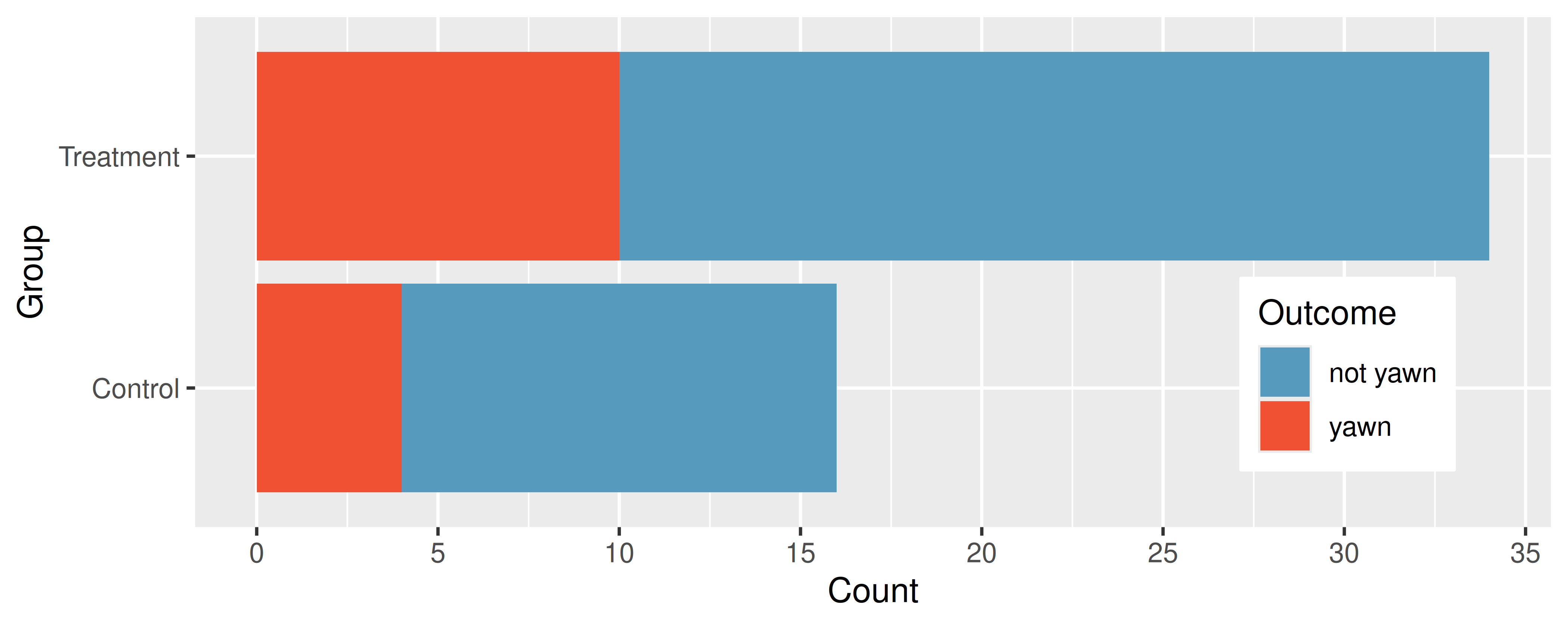
Suppose we are interested in estimating the difference in yawning rates between the control and treatment groups using a confidence interval. Explain why we cannot construct such an interval using the normal approximation. What might go wrong if we constructed the confidence interval despite this problem?

Heart transplant success. The Stanford University Heart Transplant Study was conducted to determine whether an experimental heart transplant program increased lifespan. Each patient entering the program was officially designated a heart transplant candidate, meaning that he was gravely ill and might benefit from a new heart. Patients were randomly assigned into treatment and control groups. Patients in the treatment group received a transplant, and those in the control group did not. The visualization below displays how many patients survived and died in each group. (Turnbull, Brown, and Hu 1974)

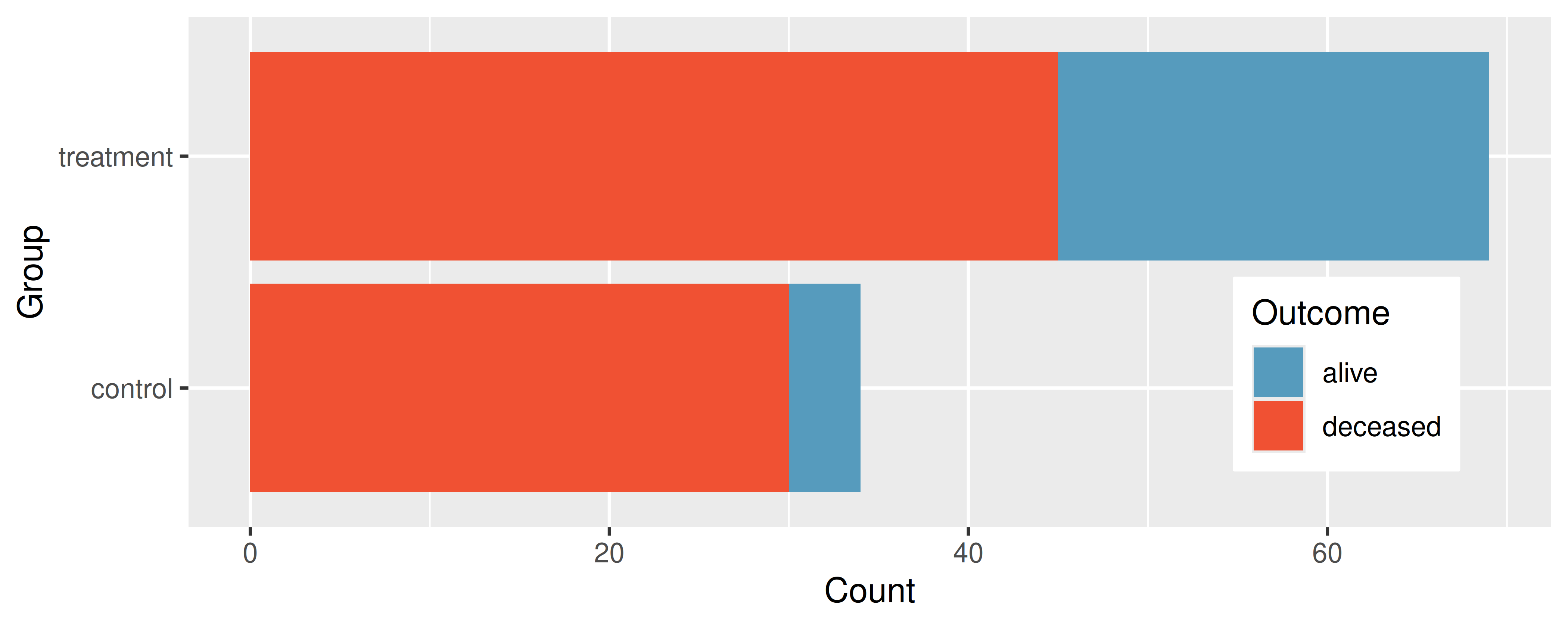
Suppose we are interested in estimating the difference in survival rate between the control and treatment groups using a confidence interval. Explain why we cannot construct such an interval using the normal approximation. What might go wrong if we constructed the confidence interval despite this problem?

Government shutdown. The United States federal government shutdown of 2018–2019 occurred from December 22, 2018 until January 25, 2019, a span of 35 days. A Survey USA poll of 614 randomly sampled Americans during this time period reported that 48% of those who make less than $40,000 per year and 55% of those who make $40,000 or more per year said the government shutdown has not at all affected them personally. A 95% confidence interval for $(p_\text{$<$40K} - p_\text{$\ge$40K})$, where $p$ is the proportion of those who said the government shutdown has not at all affected them personally, is (-0.16, 0.02). Based on this information, determine if the following statements are true or false, and explain your reasoning if you identify the statement as false. (Survey USA 2019)

At the 5% discernibility level, the data provide convincing evidence of a real difference in the proportion who are not affected personally between Americans who make less than $40,000 annually and Americans who make $40,000 annually.
We are 95% confident that 16% more to 2% fewer Americans who make less than $40,000 per year are not at all personally affected by the government shutdown compared to those who make $40,000 or more per year.
A 90% confidence interval for $(p_\text{$<$40K} - p_\text{$\ge$40K})$ would be wider than the $(-0.16, 0.02)$ interval.
A 95% confidence interval for $(p_\text{$\ge$40K} - p_\text{$<$40K})$ is (-0.02, 0.16).

Online harassment. A Pew Research poll asked US adults aged 18-29 and 30-49 whether they have personally experienced harassment online. A 95% confidence interval for the difference between the proportions of 18-29 year-olds and 30-49 year-olds who have personally experienced harassment online $(p_{18-29} - p_{30-49})$ was calculated to be (0.115, 0.185). Based on this information, determine if the following statements are true or false, and explain your reasoning for each statement you identify as false. (Pew Research Center 2021)

We are 95% confident that the true proportion of 18-29 year-olds who have personally experienced harassment online is 11.5% to 18.5% lower than the true proportion of 30-49 year-olds who have personally experienced harassment online.
We are 95% confident that the true proportion of 18-29 year-olds who have personally experienced harassment online is 11.5% to 18.5% higher than the true proportion of 30-49 year-olds who have personally experienced harassment online.
95% of random samples will produce 95% confidence intervals that include the true difference between the population proportions of 18-29 year-olds and 30-49 year-olds who have personally experienced harassment online.
We can conclude that there is a discernible difference between the proportions of 18-29 year-olds and 30-49 year-olds who have personally experienced harassment online is too large to plausibly be due to chance, if in fact there is no difference between the two proportions.
The 90% confidence interval for $(p_{18-29} - p_{30-49})$ cannot be calculated with only the information given in this exercise.

Decision errors and comparing proportions I. In the following research studies, conclusions were made based on the data provided. It is always possible that the analysis conclusion could be wrong, although we will almost never actually know if an error has been made or not. For each study conclusion, specify which of a Type I or Type II error could have been made, and state the error in the context of the problem.

The malaria vaccine was seen to be effective at lowering the rate of contracting malaria (when compared to the control vaccine).
In the US population, Asian-Indian Americans and Chinese Americans are not observed to have different proportions of current smokers.
There is no evidence to claim a difference in the proportion of Americans who are not affected personally by a government shutdown when comparing Americans who make less than $40,000 annually and Americans who make $40,000 annually.

Decision errors and comparing proportions II. In the following research studies, conclusions were made based on the data provided. It is always possible that the analysis conclusion could be wrong, although we will almost never actually know if an error has been made or not. For each study conclusion, specify which of a Type I or Type II error could have been made, and state the error in the context of the problem.

Of registered voters in California, the proportion who report not knowing enough to voice an opinion on whether they support off shore drilling is different across those who have a college degree and those who do not.
In comparing Californians and Oregonians, there is no evidence to support a difference in the proportion of each who are sleep deprived.

Active learning. A teacher wanting to increase the active learning component of her course is concerned about student reactions to changes she is planning to make. She conducts a survey in her class, asking students whether they believe more active learning in the classroom (hands on exercises) instead of traditional lecture will helps improve their learning. She does this at the beginning and end of the semester and wants to evaluate whether students’ opinions have changed over the semester. Can she used the methods we learned in this chapter for this analysis? Explain your reasoning.

An apple a day keeps the doctor away. A physical education teacher at a high school wanting to increase awareness on issues of nutrition and health asked her students at the beginning of the semester whether they believed the expression “an apple a day keeps the doctor away”. 40% of the students responded yes. Throughout the semester she started each class with a discussion of a study highlighting positive effects of eating more fruits and vegetables. She conducted the same apple-a-day survey at the end of the semester, and this time 60% of the students responded yes. Can she used a two-proportion method from this section for this analysis? Explain your reasoning.

Malaria vaccine effectiveness, effect size. A randomized controlled trial on malaria vaccine effectiveness randomly assigned 450 children intro either one of two different doses of the malaria vaccine or a control vaccine. 89 of 292 malaria vaccine and 106 out of 147 control vaccine children contracted malaria within 12 months after the treatment. (Datoo et al. 2021)

Recall that in order to reject the null hypothesis that the two vaccines (malaria and control) are equivalent, we’d need the sample proportion to be about 2 standard errors below the hypothesized value of zero.

Say that the true difference (in the population) is given as $\delta,$ the sample sizes are the same in both groups $(n_{malaria} = n_{control}),$ and the true proportion who contract malaria on the control vaccine is $p_{control} = 0.7.$ If you ran your own study (in the future), how likely is it that you would get a difference in sample proportions that was sufficiently far from zero that you could reject under each of the conditions below. (Hint: Use the mathematical model.)

$\delta = -0.1$ and $n_{malaria} = n_{control} = 20$
$\delta = -0.4$ and $n_{malaria} = n_{control} = 20$
$\delta = -0.1$ and $n_{malaria} = n_{control} = 100$
$\delta = -0.4$ and $n_{malaria} = n_{control} = 100$
What can you conclude about values of $\delta$ and the sample size?

Diabetes and unemployment. A Gallup poll surveyed Americans about their employment status and whether they have diabetes. The survey results indicate that 1.5% of the 47,774 employed (full or part time) and 2.5% of the 5,855 unemployed 18-29 year-olds have diabetes. (Gallup 2012)

Create a two-way table presenting the results of this study.
State appropriate hypotheses to test for difference in proportions of diabetes between employed and unemployed Americans.
The sample difference is about 1%. If we completed the hypothesis test, we would find that the p-value is very small (about 0), meaning the difference is statistically discernible. Use this result to explain the difference between statistically discernible and practically important findings.

Dataset sources

yawn (openintro) | heart_transplant (openintro)

StatLens Exercises

These exercises focus on the parts of inference a calculator can’t do for you: framing the question, choosing the right procedure, checking conditions, and interpreting what a tool reports. Where a link is given, let StatLens do the arithmetic and spend your effort on the reasoning.

Frame the question. A campus newspaper claims that more than 60% of students skip breakfast. A pollster surveys a random sample of 150 students and finds 99 who skip breakfast.
1. What is the parameter of interest? Describe it in words and give its symbol.
2. Write the null and alternative hypotheses in symbols. Is this a one-sided or two-sided test, and why?
3. Check the success–failure condition for using a normal-approximation $z$-procedure here.
Choose the procedure. For each scenario, name the procedure you would use — one-proportion $z$ (test or interval), two-proportion $z$ (test or interval), or not a proportion problem. You do not need to carry anything out; the skill here is matching the question to the method.
1. Is the proportion of defective parts from one assembly line different from the company’s 2% target?
2. Do a higher fraction of patients recover on a new drug than on the standard drug?
3. Is the average recovery time on the new drug shorter than on the standard drug?
4. In a single survey, estimate the percentage of voters who support a ballot measure, with a margin of error.
Check conditions before you trust the test. A medical consultant says her surgery patients have a lower complication rate than the national rate of 10%. Open the Medical Consultant data in the One-Proportion $z$-Test tool.
1. State $H_0$ and $H_A$ for the consultant’s claim.
2. The tool reports the sample size and the number of complications. Using $p_0 = 0.10$, compute $np_0$ and $n(1-p_0)$. Is the success–failure condition met?
3. Based on (b), is the normal-approximation $z$-test trustworthy here? Connect your answer to why we used a bootstrap confidence interval for this same dataset earlier in the course.
Run it and interpret it (two proportions). A randomized trial tested whether a malaria vaccine changes the infection rate. Open the Malaria vaccine trial data in the Two-Proportion $z$-Test tool.
1. Identify the explanatory and response variables, and define the parameter $p_1 - p_2$ in words.
2. State the hypotheses for testing whether the vaccine changes the infection rate.
3. Run the test. Report the 95% confidence interval for $p_1 - p_2$ that the tool gives. Does the interval contain 0?
4. Write a one-sentence conclusion in context, and say whether your confidence interval and your hypothesis test lead to the same decision.
5. Which statement is the correct interpretation of the interval in (c)?
  1. There is a 95% probability that $p_1 - p_2$ lies in this interval.
  2. If the trial were repeated many times, about 95% of the intervals built this way would contain the true difference $p_1 - p_2$.
  3. 95% of vaccinated people fall within this interval.
Simulation vs. analytic — when do they agree? The normal-approximation $z$-procedure and a simulation (bootstrap) are two routes to the same confidence interval. Sometimes they land in nearly the same place; sometimes they don’t. You will compare them on two datasets and figure out why.

First the well-behaved case. Open the Stent study data in the analytic One-Proportion $z$ tool, then open the same dataset in the bootstrap tool.
1. Record the 95% confidence interval from each tool. How close are the two intervals?
Now the troublesome case from Exercise 3. Open the Medical Consultant data in the analytic tool, then the same data in the bootstrap tool.
1. Record the 95% interval from each tool for this dataset. Are they as close as they were for the stent data? In particular, look at the shape: is the bootstrap distribution roughly symmetric, or is it skewed?
2. Explain the pattern. Why do the analytic and simulation intervals nearly coincide for the stent data but diverge for the medical-consultant data? Use the success–failure counts ($n\hat{p}$ and $n(1-\hat{p})$) from each dataset in your answer.
3. A student concludes, “Simulation and the formula disagree, so one of them must be wrong.” Why is this the wrong takeaway? Which method should you trust more when they disagree, and why?

American Council on Education. 2008. “College-Bound Students’ Interests in Study Abroad and Other International Learning Activities.” http://www.openintro.org/redirect.php?go=textbook-Interests_in_Study_Abroad_2008.

CDC. 2008. “Perceived Insufficient Rest or Sleep Among Adults – United States, 2008.” http://www.openintro.org/redirect.php?go=textbook-Perceived_Insufficient_Rest_or_Sleep_Among_Adults.

———. 2018. “2018 Assisted Reproductive Technology Fertility Clinic Success Rates Report.” https://www.cdc.gov/art/pdf/2018-report/ART-2018-Clinic-Report-Full.pdf.

Datoo, M. S., M. H. Natama, A. Somé, O. Traoré, T. Rouamba, D. Bellamy, P. Yameogo, et al. 2021. “High Efficacy of a Low Dose Candidate Malaria Vaccine, R21 in 1 Adjuvant Matrix-m$^{TM}$, with Seasonal Administration to Children in Burkina Faso.” The Lancet. https://doi.org/10.1016/S0140-6736(21)00943-0.

Demos. 2011. “The State of Young America: The Poll.” http://www.openintro.org/redirect.php?go=textbook-young_americans_2011_extra.

Gallup. 2012. http://www.openintro.org/redirect.php?go=textbook-employed_americans_in_better_health_2012.

Gallup. 2021a. “Half of College Students Say COVID-19 May Impact Completion.” https://www.openintro.org/go?id=textbook-gallup-2021-covid-college-impact.

———. 2021b. “U.s. Support for Vaccination Proof Varies by Activity, Data Collected in April 2021.” https://www.openintro.org/go?id=textbook-gallup-2021-vaccine-proof.

Kaiser Family Foundation. 2019. https://www.openintro.org/go?id=textbook-kff-2019-expand-aca-coverage.

Lo Sasso, A. T., M. R. Richards, C. F. Chou, and S. E. Gerber. 2011. “The $16,819 Pay Gap for Newly Trained Physicians: The Unexplained Trend of Men Earning More Than Women.” Health Affairs 30 (2). https://doi.org/10.1377/hlthaff.2010.0597.

Lockman, S., R. L. Shapiro, L. M. Smeaton, C. Wester, I. Thior, L. Stevens, F. Chand, et al. 2007. “Response to Antiretroviral Therapy After a Single, Peripartum Dose of Nevirapine.” New England Journal of Medicine 356 (2): 135–47. https://doi.org/10.1056/NEJMoa062876.

NORC. 2016. “Data Explorer - Government Resp to Promote Gender Equality.” https://www.openintro.org/go?id=textbook-gssdataexplorer-marijuana-gender-equality.

———. 2022. “Data Explorer - Should Marijuana Be Made Legal.” https://www.openintro.org/go?id=textbook-gssdataexplorer-marijuana-legal.

Pew Research Center. 2011. “Is College Worth It?, Data Collected March 15-29, 2011.” http://www.openintro.org/redirect.php?go=textbook-college_worth_it_2011.

———. 2021. “The State of Online Harassment, Data Collected September 8 - 13, 2020.” https://www.openintro.org/go?id=textbook-pew-2021-online-harassment.

Poll, Marist. 2011. “Road Rules: Re-Testing Drivers at Age 65?, March 4, 2011.” http://www.openintro.org/redirect.php?go=textbook-drivers_at_65_2011.

Rao, M., L. Bar, Y. Yu, M. Srinivasan, A. Mukherjea, J. Li, S. Chung, S. Venkatraman, S. Dan, and L. Palaniappan. 2021. “Disaggregating Asian American Cigarette and Alternative Tobacco Product Use: Results from the National Health Interview Survey (NHIS) 2006–2018.” Journal of Racial and Ethnic Health Disparities. https://doi.org/10.1007/s40615-021-01024-5.

Smith, G. E., P. A. Chouinard, and S. Byosiere. 2021. “If i Fits i Sits: A Citizen Science Investigation into Illusory Contour Susceptibility in Domestic Cats (Felis Silvestris Catus).” Applied Animal Behaviour Science 240. https://doi.org/10.1016/j.applanim.2021.105338.

Survey USA. 2012. “News Poll 19333, Data Collected on June 27, 2012.” http://www.openintro.org/redirect.php?go=textbook-SurveyUSA_19333.

———. 2019. http://www.openintro.org/redirect.php?go=textbook-SurveyUSA_24568.

———. 2021. https://www.openintro.org/go?id=textbook-surveyusa-2021-seattle-defund-police.

Turnbull, B., B. Brown, and M. Hu. 1974. “Survivorship of Heart Transplant Data.” Journal of the American Statistical Association 69: 74–80. https://doi.org/10.1080/01621459.1974.10480130.

Vaughn, A. 2011. “Poll Finds Young Adults Optimistic, but Not about Money.” Los Angeles Times. http://www.openintro.org/redirect.php?go=textbook-young_americans_2011.

YouGov. 2021. “Do You Think the Coronavirus Will End up Bringing the World Closer Together, or Leave Us Further Apart?” https://www.openintro.org/go?id=textbook-yougov-2021-covid.

12 Inference for Proportions

12.1 Case study: is the complication rate lower?

12.2 Building the null distribution by simulation

12.2.1 The marbles metaphor

12.2.2 From one draw to many

12.2.3 The null distribution at 1,000 simulations

12.2.4 Reading the p-value

12.3 Normal approximation for proportions

12.3.1 The sampling distribution of \(\hat{p}\)

12.3.2 The standard error of \(\hat{p}\)

12.4 Confidence interval for a single proportion

12.4.1 The formula

12.4.2 Worked example: Payday loan regulation

12.4.3 Changing the confidence level

12.5 Hypothesis test for a single proportion

12.5.1 The Z test for a proportion

12.5.2 Worked example: Support for credit checks

12.5.3 When conditions fail

12.6 Difference of two proportions

12.6.1 The parameter and point estimate

12.6.2 Confidence interval for a difference in proportions

12.6.3 Hypothesis test for a difference in proportions

12.6.4 Why pool for hypothesis tests but not for confidence intervals?

12.7 Comparing simulation-based and normal-based methods

12.7.1 An example comparison

12.7.2 When do they disagree?

12.7.3 Practical recommendation

12.8 Explore with StatLens

12.9 Chapter review

12.9.1 Summary

12.9.2 Key terms

12.10 Exercises

StatLens Exercises